ChIP-Seq Analysis Tutorial Part 2: ChIP-Seq Data Analysis

In this section, we will extend the analysis of ChIP-Seq data to:

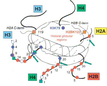
B. Analyzing histone modifications

ChIP-Seq methods can also be used for analyzing histone modification patterns at genome-scale in several organisms. There are several genome-wide approaches for profiling DNA-methylation patterns. Amongs them, ChIP combined with DNA sequencing is used for detecting patterns across the genome and providing insights into the function of histone methylation and chromatin structure. Recently, Barski et al., 2007 using ChIP-Seq have generated high-resolution maps for the genome-wide distribution of several histone methylations as well as histone variants (H2A.Z), RNA polymerase II, and CTCF across the human genome using the Solexa 1G sequencing technology. A similar application, by Mikkelsen et al., 2007, has been used for high-throughput profiling of histone modifications in the mouse cells. The two experiments have used a different procedure to treat in-vivo chromatin: in Barski et al. they treated the chromatin from human CD4⁺ cell lines with micrococcal nuclease (MNase) in order to get a detailed view of histon methylation, whereas in Mikkelsen et al. chromatin from fixed mouse ES cells was fragmented to a size range of 200-700 bases by means of a sonifier.

Both the Barski and Mikkelsen data are available on our ChIP-Seq Web site and we are now going to present a few examples of histone autocorrelation studies (using the ChIP-Cor tool) along with genome partitioning (by means of the ChIP-Part tool).

---

Methodology

A typical genome partitioning analysis involves the following steps:

1. Perform correlation studies with ChIP-Cor to evaluate the average fragment size of the ChIP-Seq data under study, and to compute the average count density in signal-rich and signal-poor regions.
2. Partition the genome into signal-rich and signal-poor regions with ChIP-Part.
3. The tag count density threshold used as a parameter for the genome partitioning algorithm is set to be twice the average tag count density outside the enriched regions.

---

1. Correlation Studies (ChIP-Cor)

We have seen in the previous example that ChIP-Cor can be used for studying the distribution of 5'-3' tag reads positions and that this gives us an estimate of the average DNA fragment size that has been precipitated by ChIP. In addition to that, ChIP-Cor is also useful to generate auto-correlation plots for different histone modifications.

Let's take as an example two different histone methylation marks in embryonic mouse cells (ES): H3K6 trimethylation and H3K4 trimethylation.

Go on our ChIP-Seq Web server at ChIP-Cor, and follow the instructions below:

On both the left and right sides under the headers ChIP-Seq Input Data (Reference Feature) and ChIP-Seq Input Data (Target Feature) make sure that the checkbox Select available Data Sets is activated. Select: Genomes : M. musculus (July 2007/mm9) on both sites. Data Type : ChIP-seq on both sides. Series : Mikkelsen 2007, histone modifications in mouse ES cells on both sides. Sample : ES H3K36me3. On both the left and right sides under the header Additional Input Data Options make sure that you select: any Strand for both the Reference and Target feature tags (any means that you correlate without distinction tags on both strands). On the input form under the header Analysis Parameters select the following values: Range. Fill in the followng values: Beginning: 0, End: 50000 It defines the relative distance between forward and reverse sequence tags reads. Window width : 10 (or 1) Count Cut-off : 1 Under Normalization options select the count density checkbox. The histogram values are in counts/bp.

You are now ready to submit the job.

Do the same for H3K4me3 .

If you compare the two auto-correlation plots for H3K36 and H3K4, you see that H3K36 shows long range correlation whereas H3K4 has short range correlation. This indicates that certain epigenetic modifications are less localized than others and bind DNA over larger regions, producing relatively broad peaks. An alternative hypothesis would be that the predominant location of H3K4me3 is close to chromosome ends (telomers). We can observe that count densities in enriched regions are 0.012 and 0.07 for H3K36 and H3K4 respectively which correspond to approximately 2 and 14 counts per nucleosome, assuming that the whole length of DNA per nuclesome is about 150-200 bps. Average count densities in signal-depleted regions are 0.005 and 0.007 for H3K36 and H3K4 respectively.

Note that with ChIP-cor you can download the numerical results as a text file which is provided as a link underneath the histogram plot. This is useful if one wants to overlay more than one plot.

As we have already mentioned, Chip-Cor is also used to study the fragment size distribution of ChIP-seq data. To this purpose, we want to compare 5'-3' correlation of H3K4me3 regions from Mikkelsen et al. with H3K4me3 from Barski et al.. As said in the previous introduction, contrary to the Mikkelsen data, the Barski data have single-nucleosome resolution.

Go to ChIP-Cor and follow the instructions below:

On both the left and right sides under the headers ChIP-Seq Input Data (Reference Feature) and ChIP-Seq Input Data (Target Feature) make sure that the checkbox Select available Data Sets is activated. Select: Genomes : H.sapiens (March 2006/hg18) on both sides. Data Type : ChIP-seq on both sides. Series : Barski 2007, CD4+ cells, histone marks on both sides. Sample : CD4+ H3K4me3 on both sides. On both the left and right sides under the header Additional Input Data Options make sure that you select: the forward (+) Strand for the Reference feature tags and the reverse (-) Strand for the Target feature tags. On the input form under the header Analysis Parameters select the following values: Range (it defines the relative distance between forward and reverse sequence tags reads). Fill in the followng values: Beginning: -500, End: 500 Window width : 10 It defines the histogram step size. Count Cut-off : 1 We count as one multiple reads that map to the same start location and orientation (since we believe that these are likely due to PCR bias). Under Normalization options select the count density checkbox. The histogram values are in counts/bp.

You are now ready to submit the job.

You can perform the same anylisis for the Mikkelsen et al. data.

As you can see from the distributions obtained from ChIP-Cor (Barski H3K4me3 and Mikkelsen H3K4me3), Mnase treatment in combination with the ChIP will lead to nucleosome-sized DNA (about 147 bp) that can be sequenced by high throughput sequencers, resulting in a fine mapping of the H3K4me3 pattern in the genome.

2. Using partitioning for analyzing differential histone modification analysis (ChIP-Part)

The partitioning model is more appropriate than peak recognition for the detection of regions or peaks of higly variable size and for differential chromatin state analysis. Histone modifications are the result of mechanisms that spread across the genome. For example, H3K36me3 is the result of trascriptional activity that leads to DNA methylation, whereas the modification H3K4me3 is associated with the transcription start site of active genes.

Our partitioning algorithm (see also the ChIP-Seq Technical Document) uses a fast dynamic programming approach to maximize a global scoring function in order to split the genome in signal-rich and signal-poor regions.

We remind that the scoring function is defined by means of two parameters, the count density threshold and the transition penalty, as the sum of scores of:

• Transitions (penalty)
• Signal-rich region scores: length x (local count-density - threshold)
• Signal-poor region scores: length x (threshold - local count-density)

We will use the ChIP-Part tool to compare H3K4me3 chromatin domains in four different mouse cell lines from Mikkelesen et al.: embryonic stem cell lines(ES and ESHyb), embryonic fibroblasts (MEF), and neural progenitors (NP).

Go to the program ChIP-Part (ChIP-Part stays for ChIP-Seq Partitioning tool) and procede as follows:

On the left side under the header ChIP-Seq Input Data activate the checkbox Select available Data Sets and select: Genomes : M. musculus (July 2007/mm9) on both sites. Data Type : ChIP-seq on both sides. Series : Mikkelsen 2007, histone modifications in mouse ES cells on both sides. Sample : ES H3K4me3. On the left side under the header Additional Input Data Options make sure that you select the any Strand option for selecting both strands. Activate Repeat Masker to filter out interspersed repeats and low complexity DNA regions. On the right side under the header Partitioning Parameters select the following values: Count Density Threshold (t) : 0.014 bp. It defines the threshold in count density for defining signal-rich regions (remember that the average count densities in regions outside peaks is 0.007) Transition Penalty (p) : -10 bp. It assigns a (negative) score to a transition from signal-rich to signal-poor region. Count Cut-off : 1 On the right side under the header Genome Viewing Parameters set the following values: BED Track Name : ES.H3K4me3 (for example)

As a rule of thumb., you can set the count density threshold to twice the average tag count density outside peak regions.

As you can see, ChIP-Part for supported species generates the following output:

• A default two-line-oriented SGA file representing signal-reach DNA regions;
• GFF, FPS, BED formats;
• A link is generated to automatically display the results on the UCSC browser as a custom annotation track;
• A statistical report with the following information:
  • Total number of processed sequences, total DNA length, and total number of fragments;
  • Total length of fragments, average fragment length, and percentage of total DNA length;
  • Percentage of total counts, average number of counts, and number of count per bp (count density).

You can try to change the partitiong parameters, such as the count density threshold or the transition penalty, in order to optimize the partitioning output.

In our case, we get 24402 fragments of average length 1778 bp.

If you click on the hyperlink to UCSC you can view the results of the partitioning program in the UCSC genome browser. On our ChIP-Seq Web server we make available a list of URLs for viewing public ChIP-Seq data as custom tracks within the UCSC genome browser. These custom tracks are provided in bigWIG format and their URLs are specified at

• /chipseq/chip_seq_wig.html

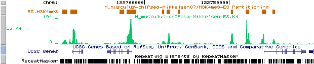
So, you can upload the track for H3K4me3 in mouse ES cells from Mikkelsen et al. and compare it with the results from the partitiong program. Here is an example of such a comparison for H3K4me3 in mouse ES cells:

Custom tracks:
Mikkelsen et al. : results of ChIP-part program (ES.K4 BED file)
ES.K4 from : http://ccg.vital-it.ch/bigWIG/mikkelsen07/ES.K4_m.BW

As we can see from these results, our partitioning model seems to fit well the data from Mikkelsen et al..

It is often useful to save the BED file generated by the partitiong program for further analysis (ES.K4.bed).

Repeat the same analysis for H3K4 in ESHyb, MEF, and NP cell lines by adjusting the count density threshold accordingly, and save the results in BED format.

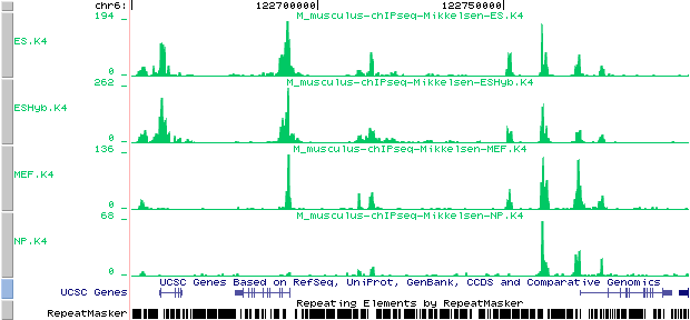
If we display the H3K4me3 profiles from Mikkelsen et al. on the UCSC browser, we can see how chromatin domains are differentially occupied in different cell lines.

Go to UCSC and proceed as follows:

• Select Assembly : "Mouse" "July 2007 (NCBI37/mm9)";
• Select Position : chr6:122,650,000-122,800,000;

and press submit to go to the genome browser. You can configure the image viewer as you wish: for this example we have just turned on the "Base Position Chromosome band", the "UCSC Genes" and "RepeatMasker" tracks, and have hidden all other tracks.

You then upload the Mikkelsen maps of chromatin state that we make available on our ChIP-Seq server (in bigWIG format) by doing the following:

• Click the "add custom tracks" button;
• Paste the URL(s)s of the data file(s) from Mikkelsen et al. (ex: http://ccg.vital-it.ch/bigWIG/mikkelsen07/ES.K4_m.BW) in the box provided and click submit;

and go to the genome browser to go back to the viewer.

Here is how the Mikkelsen annotation tracks look like on the UCSC genome browser:

Custom tracks:
Mikkelsen et al. (2007). Genome-wide maps of chromatin state in pluripotent and lineage-committed cells. Nature 448, 553-560
ES.K4 from : http://ccg.vital-it.ch/bigWIG/mikkelsen07/ES.K4_m.BW
ESHyb.K4 from : http://ccg.vital-it.ch/bigWIG/mikkelsen07/ESHyb.K4_m.BW
MEF.K4 from : http://ccg.vital-it.ch/bigWIG/mikkelsen07/MEF.K4_m.BW
NP.K4 from : http://ccg.vital-it.ch/bigWIG/mikkelsen07/NP.K4_m.BW

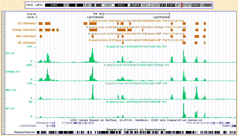
Finally, we can upload the tracks from the paritioning analysis as we have previously shown. Here are the results displayed on the UCSC browser:

Custom tracks:
Partitioning data: ES.K4.bed, ESHyb.K4, MEF.K4, NP.K4.
Mikkelsen et al. (2007). Genome-wide maps of chromatin state in pluripotent and lineage-committed cells. Nature 448, 553-560

As we can see from the results above, the ChIP-part algorithm is consistent with an intuitive interpretationof the 'count/tag' profiles of our data.