ChIP-Seq Analysis Tutorial 2
Part A: Basic task, looking at public data
(Philipp Bucher)
This tutorial explains how to use the ChIP-Seq server at:
to explore public data sets. An article describing the server and the back-end tools can be found at: Links to additional documentary material including other hands-on tutorials can be found on the home page indicated above. Note that some of the analysis steps described in this tutorial rely on programs from the Signal Search Analysis (SSA) server at: Although we will exclusively work with public data stored at the back-end of the server, it is nevertheless useful to know something about the internal data storage format, which is called SGA (Simple Genome Annotation). SGA is a compact tab-delimited text file format with five obligatory fields containing the following kinds of information:- chromosome name (e.g chr1, NC_000067.5)
- feature name (an experiment identifier)
- position (5' end of mapped sequence tag, peak center position)
- strand +, −, or 0
- count (# of tags mapping to the same position)
The "feature name" identifies the experiment. This makes it possible to merge data from different experiments into one SGA file. Fields 3-5 are more or less self-explanatory. Note however that genomic features in SGA format my be assigned orientation zero, which means "unoriented". This is appropriate for features that have no defined orientation such as peaks derived from ChIP-Seq data.
Very importantly, SGA files need to be sorted by chromosome name, position and strand, in this order of priority. This enables fast processing by the ChIP-Seq programs at the back-end of the server. For uploaded data, sorting can be delegated to the server.
This tutorial will guide you through the basic analysis tasks offered by the server. Part 1-4 deal with the analysis of ChIP-Seq data targeted at transcription factors, part 5 with histone marks.
1. Quality assessment by 5'/3' correlation analysis
Background: In a ChIP-Seq experiment targeted at a transcription factor, tags mapping to the plus and minus strand of the chromosome mark the 5' and 3' end of a transcription factor-bound DNA fragment, respectively. The minus strand tags are thus shifted with respect to the plus strand tags by a characteristic distance which is related to the average length of a pulled-down fragment and may differ between individual experiments. This global trend can be visualized by a so-called "5'/3'end correlation plot" where the relative density of minus strand tags is plotted as a function of the distance from nearby plus strand tags. At the same time, such a plot also provides an estimate of the signal-to-noise ratio and reveals common artifacts.
The proposed exercise is based on data from Chen et al. 2008 deposited in GEO entry GSE11431. This series contains data from ChIP-Seq experiments carried out to map in vivo binding sites of 15 different transcription factors in mouse embryonic stem cells.
Step-by-step procedure: Let's make a 5'/3' correlation plot for the ES Nanog data set generated in the preceding part. To this end, open the ChIP-Seq server home page in a new window:
and select "ChIP-cor" from the main menu displayed on the left side. Fill out the form as follows:
Input Data Reference Feature: Input Data Target Feature: x Select available Data Sets x Select available Data Sets Genome: M. musculus (July 2007... Genome: M. musculus (July 2007... Data Type: ChIP-Seq Data Type: ChIP-Seq Series: Chen 2008, ES cells ... Series: Chen 2008, ES cells ... Sample: ES Nanog Sample: ES Nanog Additional Input Data Options Additional Input Data Options Strand: + Strand: - Centering: (blank) Centering: (blank) Repeat Masker: unchecked Repeat Masker: unchecked Analysis Parameters Input Range : -1000 to 1000 Histogram Parameters Window width: 10 Count Cut-off value: 1 Normalization: count density |
On the output page, you will see the following picture:
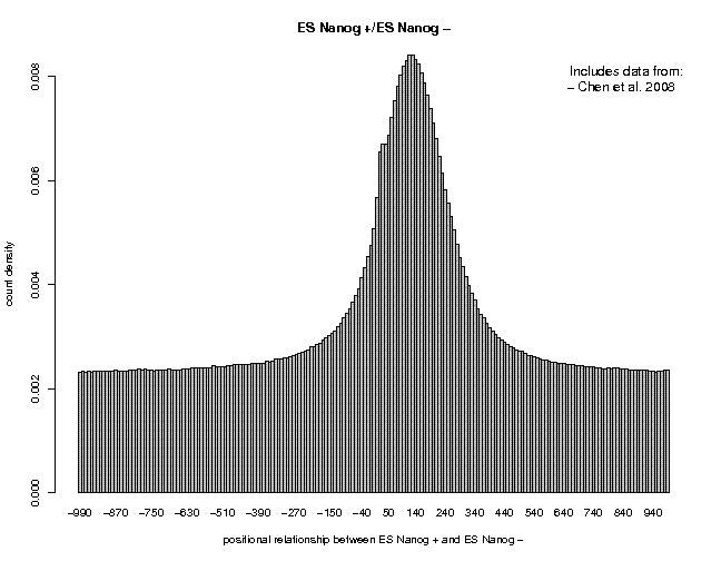
The picture shows a near-Gaussian peak centered at about position +130. On the left side, there is a weak shoulder at about position +35 which results from a common artifact seen in almost all ChIP-Seq experiments. Below the figure are a number of links: Clicking on "TEXT" enables you to download the numerical values from which the figure was produced. The link "Single Gaussian Fit" takes you to a figure showing an optimal Gaussian fit and the corresponding parameters (the parameter μ is the peak center position, here μ = 129).
The peak center position is an important parameter of the data, because we will use "centered" data in most subsequent analysis steps. Centering means shifting the positions of tags mapping to the + or − strand of the chromosome by a fixed distance downstream and or upstream, respectively. Centering increases the resolution of the ChIP-Seq data. The optimal centering distance is μ/2. Note that the relative shift between + and − tags varies from one experiment to another.
Let's now look at two other datasets from the same series:
   ES Smad1
   ES CTCF
The results are shown below:
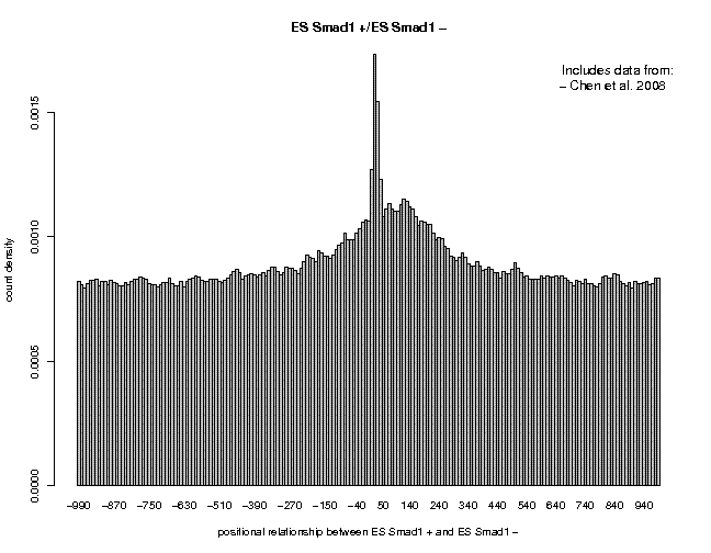
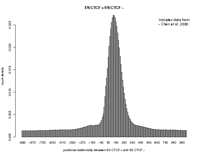
Smad1 is a low-quality data set. The prominent peak located at 35 a is a known artifact. The peak center at about 150 has a very low signal-to-noise ratio. In Contrast, the CTCF data are of very high quality. The signal-to-noise ratio is better than for Nanog. Feel free to look at other data sets from the same or a different series.
2. Peak-calling with the ChIP-Seq server
Background: The ChIP-seq server offers a basic peak finding tool called ChIP-Peak for ChIP-Seq data. It is certainly not the most advanced tool, but it is fast and easy to use. We will test ChIP-Peak with the ES Nanog data set.Step-by-step procedure: It is recommended to use centered ChIP-Seq tags as input. From the previous 5'/3' correlation analysis, we know that the optimal centering distance is 65. ChIP-Peak has two additional parameters that need to be fine-tuned to a specific data set: The window width and the threshold number of sequence tags per peak. We can obtain reasonable estimates for these parameters by re-running ChIP-cor with centered tags:
Input Data Reference Feature: Input Data Target Feature: x Select available Data Sets x Select available Data Sets Genome: M. musculus (July 2007... Genome: M. musculus (July 2007... Data Type: ChIP-Seq Data Type: ChIP-Seq Series: Chen 2008, ES cells ... Series: Chen 2008, ES cells ... Sample: ES Nanog Sample: ES Nanog Additional Input Data Options Additional Input Data Options Strand: any Strand: any Centering: 65 Centering: 65 Repeat Masker: unchecked Repeat Masker: unchecked Analysis Parameters Input Range : -1000 to 1000 Histogram Parameters Window width: 10 Count Cut-off value: 1 Normalization: count density |
The results page shows a peak centered at zero. Below the figure is a link "Parameters". Clicking on this link displays the following text:
Single Gaussian Fit Parameters Formula: y ~ a + (b/(sig*sqrt(2*pi))) * exp(-(x - mean)^2/(2 * sig^2)) Estim. SE t Pr(>|t|) a 0.00495 2.63e-05 188 2.81e-222 b 3.27 0.0287 114 1.78e-180 sig 112 1.01 110 9.46e-178 mean 0.502 0.948 0.529 0.597 Residual = 0.01065 Peak Finding Parameters Estimate Av. BG density (cnts) 0.00495 Peak window width (bp) 224 Peak threshold (cnts) 8 Peak Threshold Expected Random Peaks 5 11857 6 1835 7 250 8 30 |
In the lower part, we find recommended parameters for ChIP-Peak. The window width of 224 is based on the estimated sigma of the Gaussian fit. The peak threshold of 8 is based on the number of expected random peaks in the entire genome. We will use these parameters with ChIP-Peak. Go to the input form at:
and fill it out as follows:
ChIP-Seq Input Data                 Peak Detection Parameters

x Select available Data Sets          Window Width (bp): 224
                                      Vicinity Range (bp): 224
  Genome:  M. musculus (July 2007..   Peak Threshold: 8
  Data Type: ChIP-Seq                 Count Cut-off: 1
  Series: Chen 2010, ES cells, ...    Refine Peak Positions: checked
  Sample: ES Nanog
                                    Genome Viewing Parameters
Additional Input Data Options
                                      WIG Track Name: unchecked (blank)
  Strand: any                         Chromosome Region: unchecked (blank)
  Centering: 65
  Repeat Masker (unchecked)
|
On the output page, we can see that 26614 were detected. The authors of the paper reported 10343 peaks. To get a comparable number, we rerun ChIP-peak with a peak threshold of 15. No we get 10087 peaks.
The output is provided in two formats, SGA and FPS. The latter is the format requered by the Signal Search Analysis server, which will be used in the next part. Save the two files under the names ES_Nanog_chippeak.sga and ES_Nanog_chippeak.fps. The files can be found here:
Below the links is a small input form that enables you to extract the sequences around the peak regions in Fasta format. You may use this tool to extract sequence sets for motif analysis (see part 4).3. Evaluation of peak lists by motif enrichment and positional distribution
Background: The enrichment in DNA sequence motifs known to be bound by the factor (through direct or indirect interactions) is a useful proxy to assess the quality of peak collections obtained with different peak finders (or with different parameter combination of the same peak finder). We will use this criterion to compare our Nanog peak collection with the peak collection deposited by the authors of the data in GEO. The latter is available from the ChIP-Seq server menu under the name "ES Nanog Peaks". According to the authors, the dominant motif in Nanog peak regions is the octamer motif ATGCAAAT. Nanog itself reportedly recognizes a motif with consensus sequence CCATCA.For motif enrichment analysis, we will use the program OProf from the signal Search Analysis Server (Ambrosini et al. 2003). This programs generates a graph showing the frequency of a particular sequence motif at at relative distances from a so-called "functional site", in our case Nanog binding sites defined by a ChIP-Seq experiment.
Step-by-step procedure
Go to:
and choose "OProf" on the left side of the page under "Access to SSA Tools". Then fill out the input form as follows:
SSA Input Data                       Signal Description

  x Upload FPS File                    x consensus seq: ATGCAAAT

  ES_Nanog_chippeak.fps                Name: ATGCAAAT
  FPS name: ChIP-peak                  Reference position: 4
  FPS type: Nanog peak
                                       Cut-off:
Sequence Range
                                       x mismatches: 1
  Entire sequence range: unchecked
  5'border: -999  3'border: 1000

Sliding window parameters

  Window size: 50 Window shift: 5
  Search mode: bidirectional
|
The fields "FS name", "FPS type" and "Name" (on the right side) only define text elements displayed in the output figure. They do not influence the analysis in any other ways. We use the search mode "bidirectional" because ChIP-Seq peak are unoriented. In the output, you can see a clear peak centered at position 0.
To repeat the same type of analysis with the peak list provided by the authors, we have to export the list from the ChIP-Seq server. Currently the simplest way to do this is by using the ChIP-peak interface, although this tool was not designed for this purpose. Go to:
and fill it out the form as follows:
ChIP-Seq Input Data                 Peak Detection Parameters

x Select available Data Sets          Window Width (bp): 1
                                      Vicinity Range (bp): 1
  Genome:  M. musculus (July 2007..   Peak Threshold: 1
  Data Type: ChIP-Seq                 Count Cut-off: 1
  Series: Chen 2010, ES cells, ...    Refine Peak Positions: unchecked
  Sample: • ES Nanog peaks
                                    Genome Viewing Parameters
Additional Input Data Options
                                      WIG Track Name: unchecked (blank)
  Strand: any                         Chromosome Region: unchecked (blank)
  Centering: (blank)
  Repeat Masker (unchecked)
|
Save the output files under the names ES_Nanog_peaks.sga and ES_Nanog_peaks.fps. A copy of these files can be found here:
Now use OProf as before to evaluate this peak list by the motif enrichment test. To exactly reproduce the figures shown, enter "From Chen08" as FPS name. The motif occurrence profiles obtained with the two peak lists are shown below.
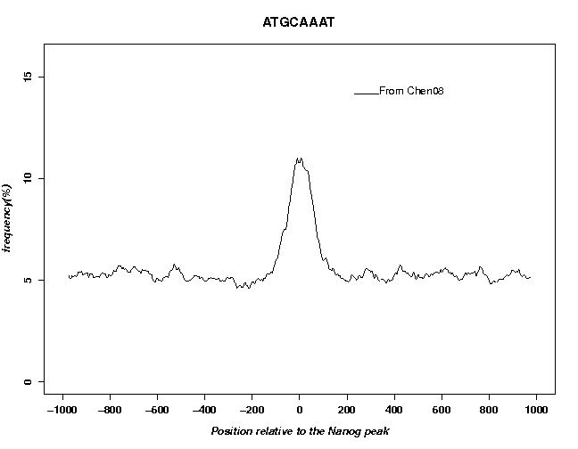
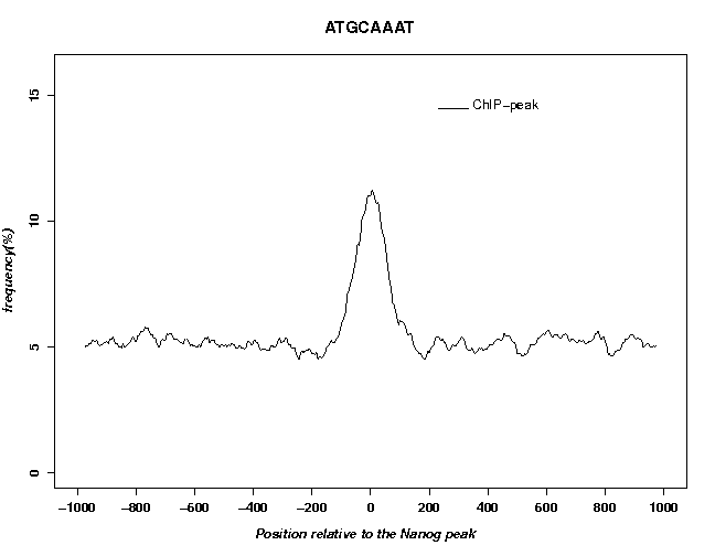
The two profiles look similar indicating that the two peak lists are roughly equivalent.
Where to go from here: You may repeat this analysis with the true Nanog binding motif CCATCA. Choose zero mismatches instead of one with this shorter consensus sequence. You may also rerun ChIP-Peak with other parameters, for instance a lower or higher peak threshold, or with different window width. Alternatively, you may repeat this exercise with the data for Sox2, Smad1 or Oct4 from the same series. The peak lists for these factors were reported to be enriched in octamer motifs as well.
4. Motif discovery in ChIP-Seq peaks
Background: The motif enrichment test exemplified in the previous exercise can only be carried out if an expected binding motif is known. If this is not the case, an over-represented sequence motif needs to be found first. The Signal Search Analysis server offers two tools to this end: SList and PatOp. These tools are powerful in that they can process large data sets in short time. However, they are not the easiest programs to use. We therefore propose to use an external progran, MEME-ChIP from the MEME Suite (Bailey et al. 2009).Since MEME-ChIP is relatively slow and can only process a limited number of sequences, we will only use about 300 top-ranked peaks, i.e. those with the highest tag coverage. We will also limit the length of the extracted sequences to 100 bp. We could extract such a sequence set by using ChIP-Peak again with a higher threshold. However, we can achieve the same by using a special post-processing feature of ChIP-Cor as illustrated by the following recipe.
Motif discovery programs can be misguided by common repetitive elements that make up a large fraction of mammalian genomes. To prevent MEME-ChIP from reporting parts of repetitive elements as over-represented motifs, we will enable repeat masking in the following exercise. This will filter out on input all ChIP-Seq tags or peaks that fall into annotated repeat regions. The filtering tools is based on the RepeatMasker track from the USCS genome browser database.
Step-by-step procedure: Go to the ChIP-Cor page at:
and fill out the form as follows:
ChIP-Seq Input Data (Reference): ChIP-Seq Input Data (Target): x Upload Custom Data x Select available Data Sets Pleas select format: SGA Genome: M. musculus (July 2007.. from File: ES_Nanog_chippeak.sga Data Type: ChIP-Seq from URL: (blank) Series: Chen 2008, ES cells ... Sorting input: off Sample: ES Nanog Experiment: Nanog peaks Feature: blank Genomes: M. musculus (July 2007.. Additional input options: Additional input options: strand: any strand: any Centering: (blank) Centering: 65 Repeat Masker: checked Repeat Masker: unchecked Analysis parameters: Input range: -1000 to 1000 Histogram Parameters Window width: 10 Count Cut-off value: 1 Normalization: count density |
Note: The input field "Experiment" accepts text that will be displayed in the output. The input field "Feature" allows selecton of lines from the SGA file based on the feature field. It should be left blank if all lines should be read or if the internal feature names are unkown. "Sorting input" should be switched on only if the input file is not properly sorted (see) ChIP-Seq Technical Document. Otherwise, sorting is a waste of time.
On the ChIP-Cor results page, we see (as expected) a high peak centered at 0. At the bottom of the page appears a new menu which we fill out as follows:
Enriched Feature Extraction Option x From: -112 To: 122 x Threshold: 100 x Cut-off: 1 Switch to Depleted Feature Extraction: off Ref Feature Oriented: off x Genomes: Mus musculus (July 2007) |
This returns of peak list of 273 sites, approximately the number we were targeting. In general, the threshold needs to be adjusted by trial and error.
Now, turn to the menu "Sequence Extraction Option" and extract sequences from -50 to 50. A new link "Sequence File" will appear. Open this link.
Now, open the home page of the MEME Suite in another browser window:
and click on the MEME-Chip link near the lower right corner of the page. Enter your email address, then copy&paste the sequences from the open ChIP-Cor window into the text area of the MEME-ChIP page that serves for sequence input. Don't change any of the proposed default parameters. Click on the "start search" button.This may take some time, especially if several people launch a job at the same time. If you are impatient, you can look at a recently generated results page at the following link:
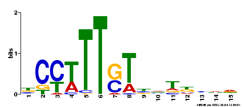
On the MEME-ChIP result page, click on the link "HTML" in the table row starting with "MEME output". Surprisingly, the most prominent motif found by MEME does not resemble the motifs described in previous publications:
E-value 3.1e-049 Width 15 Sites 273 |
|
We will test whether this motif is indeed over-represented near Nanog sites found by ChIP-Peak. To this end, we have to extract the motif in position weight matrix format. Below the graphical display of motif 1, you will find a line starting with title "Data Formats". There, click on the link "PSSM format". The following scoring will appear:
Sequence Input                       Signal Description

  x Upload FPS File                    x Weigh matrix:

  .../ES_Nanog_chippeak.fps              (cu&paste matrix from MEME
  FPS name: ChIP-peak                     output into text area
  FPS type: Nanog peak                    without header line)

Sequence Range                         Name: MEME motif 1
                                       Reference position: 8
  Entire sequence range: unchecked
  5'border: -999  3'border: 1000       Cut-off:

Sliding window parameters              x percentage: 96

  Window size: 50 Window shift: 5
  Search mode: bidirectional
|
Submit!
The resulting motif occurring profile is shown below together with the previously obtained profile obtained for the octamer consensus sequence ATGCAAAT.
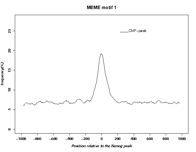
The motif found by MEME looks better. The peak is almost twice as high whereas the background frequency is only slighly higher than with the consensus sequence ATGCAAAT. Note that the cut-value (expressed as a percentage of the range between lowest and highest possible score) has been chosed such as to approximately match background frequency of the octamer consensus sequence.
The biological interpretation of this finding remains speculative. Nanog is perhaps in most cases indirectly recruited to its target sites via protein-protein interactions with other DNA-binding proteins such as Oct4. The motif found by MEME may be the recognition sequence of yet another interaction partner of Nanog.
5. 5'/3' correlation analysis for histone marks
Background: Antibodies against histone modifications (e.g. H3K4me3) or histone variants (e.g. H2AZ) pull down nucleosomes. A nucleosome covers about 145 bp of DNA. In principle the +/− strand tag shift should be in the same order or perhaps somewhat longer. However, we expect to see such a shift only if nucleosomes are positioned in the same way in all cells, which may not be the case for all regions of the genome. Moreover, histone marks tend to be more evenly distributed along the genome, resulting in ia less favorable local signal-to_noise ratio. The consequence of these circumstances is that the +/− strand tag shift is more difficult to determine for marks. Note further that 5'/3' correlation plots for histone mark often show an oscillatory pattern with a period of about 200 bp, reflecting the inherent periodicity of chromatin structure.An alternative way to determine the optimal cenetering distance for ChIP-Seq data against histone marks exploits the fact that promoters have a rigidly positioned +1 nucleosome centered at about position +120. If we generate a correlation plot with a collection of transcription start sites (TSS) as reference feature and either + or − strand tags from a ChIP-Seq experiment against histone marks as target feature, we should in principle see a peak corresponding to the +1 nucleosome. The relative shift of the peaks seen with the + and − strand tags indicates the optimal centering distance.
There are two types of ChIP-Seq protocols used for histine marks, one using MNase digestion for fragmentation, the other one using sonication. MNase digestion resolves nucleosome positions at higher resolution. MNase digestion alone (without prior immunoprecipitation) can be used to generate nucleosomal maps for a given cell type. In the following exercsise, we will use classical data sets representing the three different types of experiments:
- ChIP/sonication: Histone marks in mouse ES cells ( Mikkelsen et al. 2007)
- ChIP/Mnase: Histone marks in human CD4+ T-cells ( Barski et al. 2007)
- Mnase only: Nucleosome maps for human CD4+ T-cells ( Schones et al. 2008)
We will further use TSS collections from two sources:
-
Ensembl
at
http://www.ensembl.org/index.html
EPDnew at http://www.ensembl.org/index.html
Step-by-step procedure: We will first analyse histone marks in mouse embryonic stem cells. Open the ChIP-Cor page in another window:
and provide the following input:
Input Data Reference Feature: Input Data Target Feature: x Select available Data Sets x Select available Data Sets Genome: M. musculus (July 2007... Genome: M. musculus (July 2007... Data Type: ChIP-Seq Data Type: ChIP-Seq Series: Mikkelsen 2007, histone... Series: Mikkelsen 2007, histone... Sample: ES H3K4me3 Sample: ES H3K4me3 Additional Input Data Options Additional Input Data Options Strand: + Strand: - Centering: (blank) Centering: (blank) Repeat Masker: unchecked Repeat Masker: unchecked Analysis Parameters Input Range : -1000 to 1000 Histogram Parameters Window width: 10 Count Cut-off value: 1 Normalization: count density |
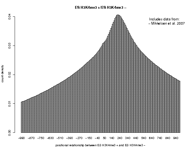
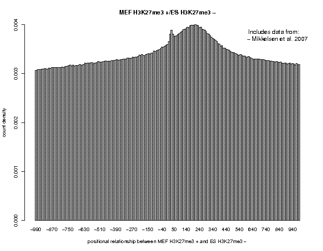
We see a single peak centered near 200. The output page indicates that the Gaussian fit has failed. If we fillow the link "TXT", we can see that the maximum − strand tag frequency occurs at position 220, indicating that we whould use a centering distance of 110 for this data set. Now, repeat the analysis sample "ES H3K27me3" from the same series. We see a flatter peak centered at 210. The two correlation plots are shown below.
Now let's look at the distribution of the H3K4me3 near promoters. To this end, fill out the ChIP-Cor form as follows:
Input Data Reference Feature: Input Data Target Feature: x Select available Data Sets x Select available Data Sets Genome: M. musculus (July 2007... Genome: M. musculus (July 2007... Data Type: Genome Annotation Data Type: ChIP-Seq Series: EPD, the Mouse curated ... Series: Mikkelsen 2007, histone... Sample: TSS from EPD New rel. 1.0 Sample: ES H3K4me3 Additional Input Data Options Additional Input Data Options Strand: oriented Strand: + Centering: (blank) Centering: (blank) Repeat Masker: unchecked Repeat Masker: unchecked Analysis Parameters Input Range : -2000 to 2000 Histogram Parameters Window width: 10 Count Cut-off value: 1 Normalization: count density |
Note that we changed the input range to "-2000 to 2000". The Strand feature "oriented" has the effect that the target feature distributions will be inverted for transcription start sites that are located on the − strand of the chromosome.
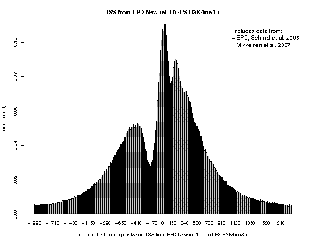
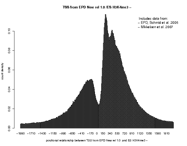
In the resulting 5'/3' correlation plot, we see a shart peak centered at about +35. A second peak center at 200 is also visible, indicating the beginning of th +2 nucleosome. Now generate the same plot for the − strand tags of the same sample. There, the first peak is centered at about position "+25, suggesting a 5'/3' shift of 190, somewhat lower than the estimate from the autocorrelation analysis. Finally, generate once again the same type of plot, this time with centered ChIP-Seq tags. A centering distance of 100 may be a good compromise from the two estimates. This time, the peak corresponding to the +1 nucleosome is centered at pos. +130, close to the expected position. The three plots resulting from these analyses are shown below.
|
|
|
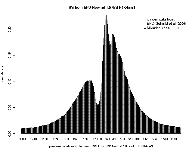
Note that H3K4me3 is typical promoter histone mark which is highly enriched in promoter-associated nucleosomes. Therefore we have high local tag coverage near trascription start sites resulting in sharp peaks. You may repeat this exercise with other histone marks, for instance H3K27me3. You will see a far more fuzzy picture. You could also repeat the analysis with the Ensembl TSS instead of the EPD collection:
   Series: ENSEMBL59, TSS collection
   Sample: TSS from ENSEMBL59
The overall picture will be the same, but the two downstream peaks will be lower and not so well seperated from each other.
Let's now repeat the same analysis with histone modification data for human CD4+ T cells. Use the following data for this purpose:
   Genome: H. sapiens (March 2006/hg18)

   Data: ChIP-Seq
   Series: Barski 2007, CD4+ cells, histone marks
   Sample: "CD4+ H3K4me3", CD4+ H3K27me3"

   Data: Genome Annotation
   Series: EPD, the Human Curated Promoter Database
   Sample: "TSS from EPD New rel 1.0
   Series: ENSEMBL52, TSS collection
   Sample: TSS from ENSEMBL52
First, let's look at the 5'/3' correlation plots for H3K4me3 and H3K27me3:
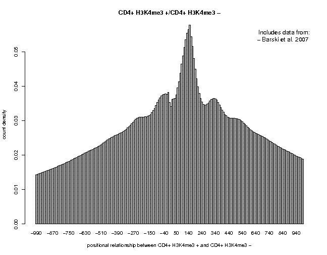
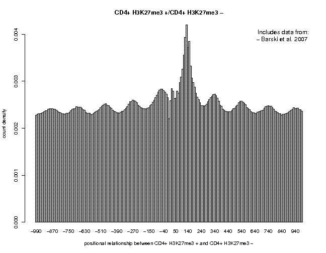
In this profiles, the major peak is centered around pos. +140, very close to the size of a nucleosome. Moreover, we see an oscillatory pattern, particularly impressive for H3K427new.
Below are correlation plots showing the distribitution of H3K4me3 ChIP-Seq tags around TSS.
|
|
|
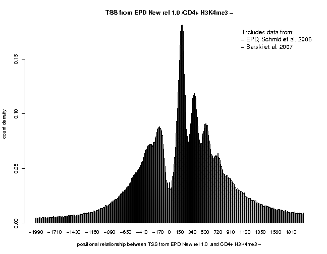
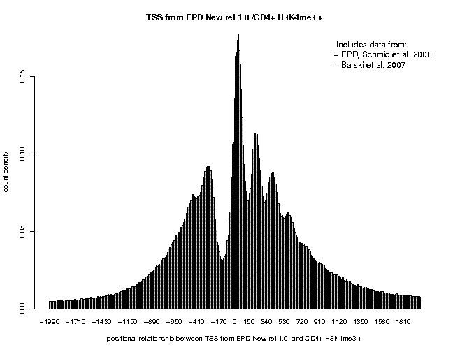
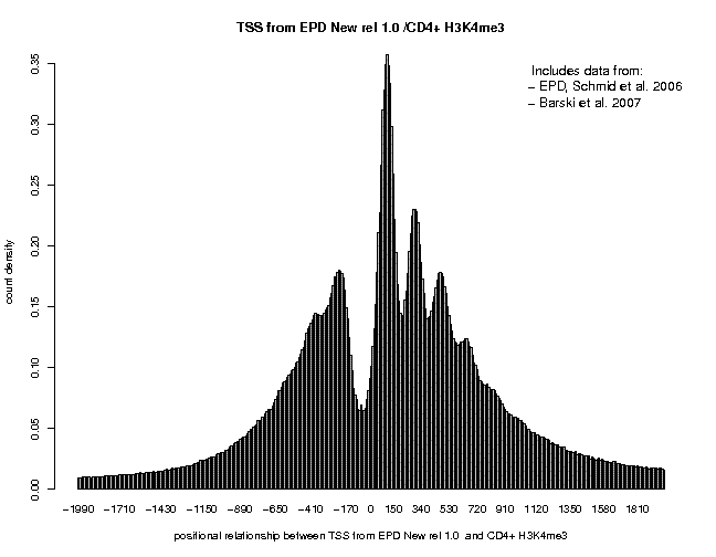
In general, the peaks are higher and cleaner supporting the claim that MNase treatment maps nucleosomes at higher resolution that sonication. The peaks obtained with the + and − strand tags are centered at positions +35 and +185. The major peak obtained with centered tags (centering distance 70) is located at pos. +110.
Finally, let's look at the distribution of nucleosomes defined by MNase digestion in promoter regions. Use the following data for this purpose.
   Genome: H. sapiens (March 2006/hg18)
   Data: ChIP-Seq
   Series: Schones 2008, CD4+ cells, nucleosome profiling, GSE10437
   Sample: CD4+ activated nucleosomes

   Data: Genome Annotation
   Series: EPD, the Human Curated Promoter Database
   Sample: "TSS from EPD New rel 1.0
Below is the picture obtained with centered MNase tags using a centering distance of 70. Note that this analysis takes longer because the MNase data sets are very big. To cover every nucleosome of the human genome by about 10 sequence tags, a total of about 150 million tags is required.
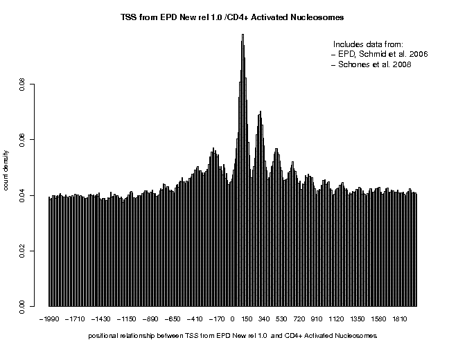
We see essentially the same nucleosome positioning pattern, however with no particular enrichment in the promoter region. In the downstream region, we see an oscillatory pattern extending over at least 7 nucleosomes.

