ChIP-Seq Analysis Tutorial 2
Part C: Advanced applications
(Philipp Bucher)
This tutorial explains how to use the ChIP-Seq server at:
to explore public data sets. An article describing the server and the back-end tools can be found at: Links to additional documentary material including other hands-on tutorials can be found on the home page indicated above. Note that some of the analysis steps described in this tutorial rely on programs from the Signal Search Analysis (SSA) server at: Although we will exclusively work with public data stored at the back-end of the server, it is nevertheless useful to know something about the internal data storage format, which is called SGA (Simple Genome Annotation). SGA is a compact tab-delimited text file format with five obligatory fields containing the following kinds of information:- chromosome name (e.g chr1, NC_000067.5)
- feature name (an experiment identifier)
- position (5' end of mapped sequence tag, peak center position)
- strand +, −, or 0
- count (# of tags mapping to the same position)
The "feature name" identifies the experiment. This makes it possible to merge data from different experiments into one SGA file. Fields 3-5 are more or less self-explanatory. Note however that genomic features in SGA format my be assigned orientation zero, which means "unoriented". This is appropriate for features that have no defined orientation such as peaks derived from ChIP-Seq data.
Very importantly, SGA files need to be sorted by chromosome name, position and strand, in this order of priority. This enables fast processing by the ChIP-Seq programs at the back-end of the server. For uploaded data, sorting can be delegated to the server.
Part 1 and 2 illustrate some of the more advanced or specialized applications of the ChIP-Seq and SSA servers. Part 3 shows how a complex analysis task can be achieved by running several programs in a pipeline.
1. Visulaizing promoter enrichment with correlation plots
Background: Some transcription factors preferentially bind to promoter regions, others tend to occur at distant enhancers. The enrichment of binding sites in promoter regions can be visualized with correlation plots, in which the frequency of the target feature (either ChIP-Seq tags or peaks) is plotted relative to the position of nearby transcription start sites(TSS). The ChIP-Seq server provides TSS collections to this end. We will illustrate the phenomenon of promoter enrichment with two contrasting examples from the Chen et al. 2008 data set: Nanog which prefers distal enhancers and c-Myc which predominantly binds to promoters.Step-by-step procedure: Go to the ChIP-Cor page at: /chipseq/chip_cor.php and fill out the form as follows:
Reference Feature: Target Feature: x Select available Data Sets x Select available Data Sets Genome: M. musculus (July 2007.. Genome: M. musculus (July 2007.. Data Type: Genome Annotation Data Type: ChIP-Seq Series: ENSEMBL59, TSS collection Series: Chen 2010, ES cells, ... Sample: TSS from ENSEMBL59 Sample: ES Nanog Additional Input Data Options: Strand: oriented Strand: any Centering: blank Centering: 65 Repeat Masker: unchecked Repeat Masker: unchecked Analysis parameters: Input Range : -5000 to 5000 Window width: 20 Count Cut-off value: 1 Normalization: global |
Look at the result, then repeat the same analysis with sample "ES c-Myc" as target feature. The resulting plots are shown below.
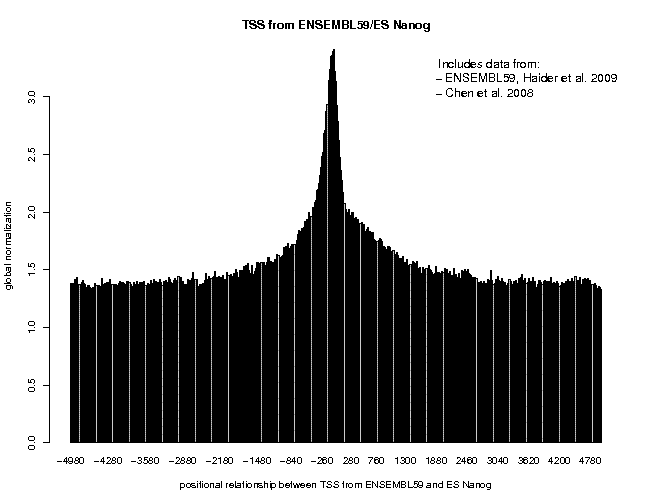

The normalization mode "global" chosen for this analysis causes the program to display the target feature frequency as "fold increase over the genome average". This allows for direct comparison of the enrichment between different experiments. We observe an approximately 3-fold and 6-fold enrichment for the two factors, respectively. These values may not be totally representative of true binding events as promoter regions have an open chromatin structure and therefore have generally tendency to "attract" ChIP-seq tags. (It may be informative to repeat the analysis with the sample "ES GFP/control".)
Let's now repeat this analysis for the extracted binding site peaks. We will use the peak collections provided by the authors via GEO. To carry out this analysis, use the samples "ES Nanog peaks" and "ES c-Myc peaks", delete the number in the "Centering" field and increase the window width to 100. You will get the following figures.
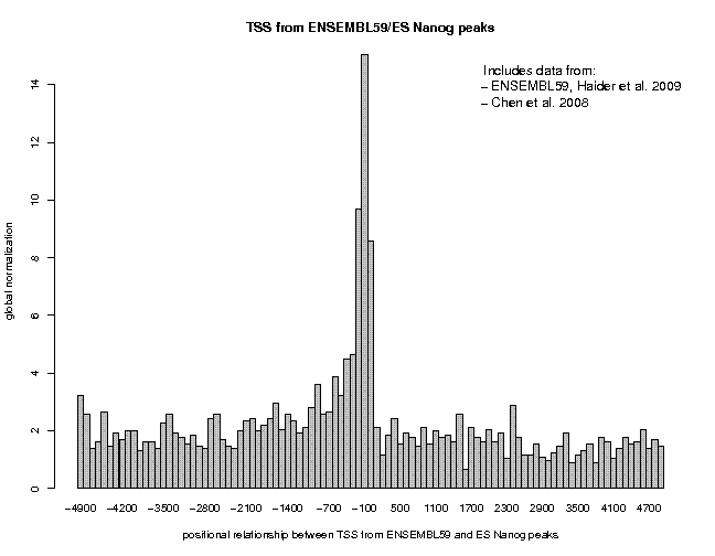
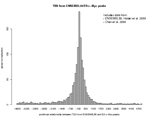
Now we can see a more pronounced difference. c-Myc peaks are 180-fold over-represented near promoters, Nanog peaks only 14-fold. We also notice a difference in peak location and shape. Nanog shows a narrow and asymmetrical peak confined to the upstream region. c-Myc shows a broader symmetrical peak extending into the downstream region.
2. Analysing the genomic and epigenomic context of transcription factor binding sites with ChIP-cor
Background: In vivo transcription factor binding sites often occur in a specific chromatin context which can be described in terms of nucleosome positioning and histone modifications. ChIP-Seq data for histone modifications in mouse ES cells and other cell types have been published by Mikkelsen et al. 2007. and Creyghton et al. 2010. These data sets have been installed at the back-end of the ChIP-Seq server. We will look at the distribution of histone marks H3K4me3, H3K4me1, and H3K27ac around three transcription factors (Nanog, c-Myc, and CTCF) in ES cells. The three histone marks were reported to be enriched in different functional regions of the genome: H3K4me3 in promoters, H3K4me3 at poised and active enhancers, H3K27ac only at active enhancers.The ChIP-seq server also offers cross-genome conservation counts derived from the UCSC PHASTCONS track available at:
In vivo binding sites are supposed to be more conserved than the corresponding flanking regions. Moreover, the size and the shape of the conservation peaks may tell us something about the mode of action of the transcription factor. We will illustrate cross-genome conservation profile analysis with the same three transcription factors that were used for chromatin context analysis.Step-by-step procedure: Use ChIP-cor with the following input specifictions in order generate an enrichment profile for H3K4me3 around Nanog binding sites:
Reference Feature: Target Feature: x Select available Data Sets x Select available Data Sets Genome: M. musculus (July 2007.. Genome: M. musculus (July 2007.. Data Type: ChIP-Seq Data Type: ChIP-Seq Series: Chen 2010, ES cells, ... Series: Mikkelsen 2007, histone ... Sample: ES Nanog peaks Sample: ES H3K4me3 Additional Input Data Options: Strand: any Strand: any Centering: blank Centering: 100 Repeat Masker: unchecked Repeat Masker: unchecked Analysis parameters: Input Range : -2500 to 2500 Window width: 50 Count Cut-off value: 1 Normalization: global |
Look at the result, then repeat the same analysis with samples "ES c-Myc peaks" and "ES CTCF peaks" as reference features, and with samples "ES H3K4me1" and "ES H3K27ac/rep1" from the series "Creyghton 2010, histone marks ..." as target features. The 9 resulting plots are shown below.
|
|
|
|
|
|
|
|
|
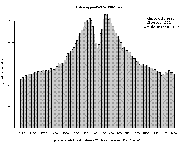
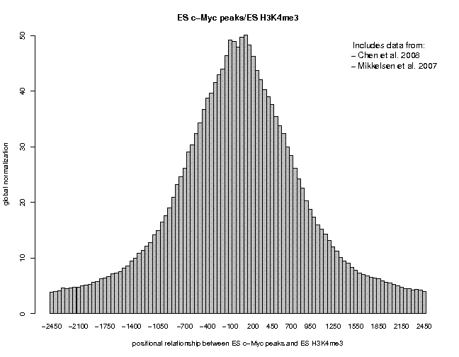
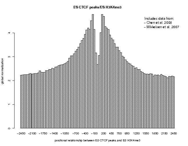
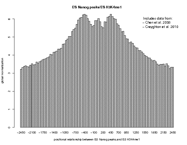
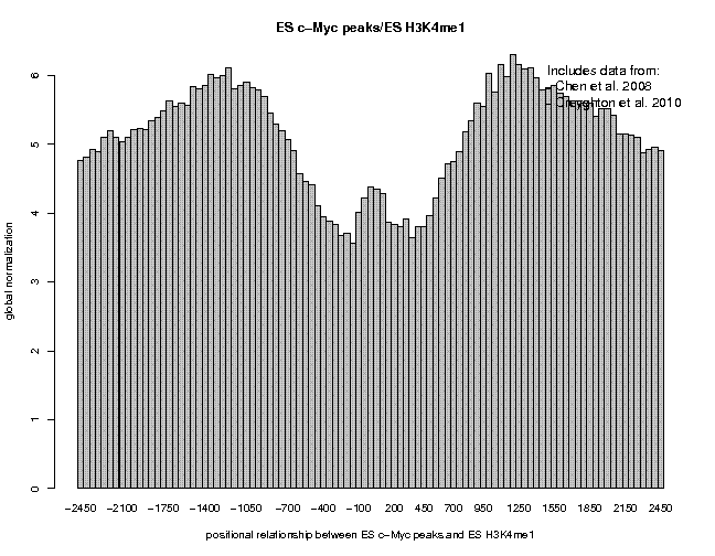
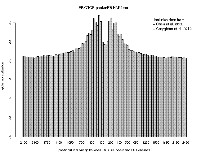
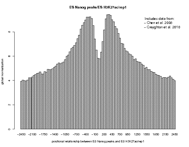
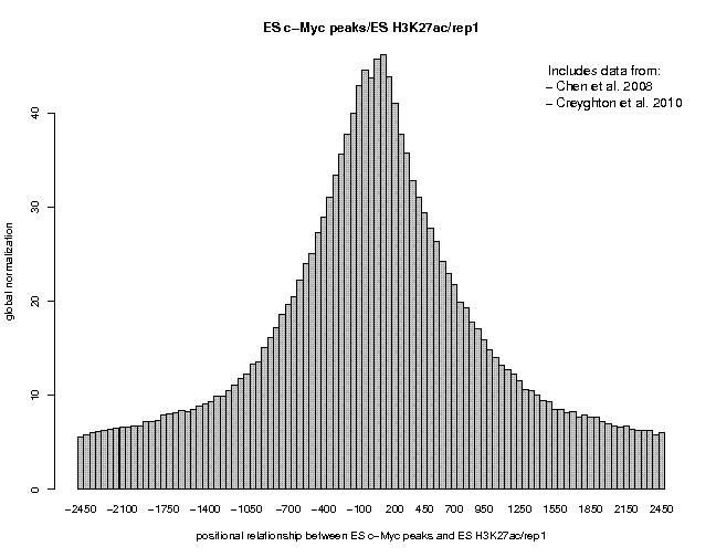
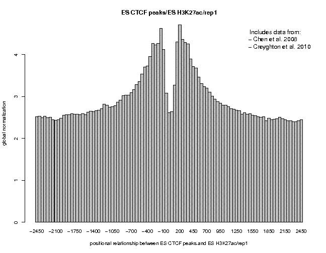
Many observations can be made in these figures. In general we see broad enrichment in histone marks around the site and often a narrow valley directly at the site. The local minimum at the sites presumably reflects a nucleosome-free region. For H3K4me1, we see a small peak exactly co-localizing with Nanog and c-Myc sites. This peak could come from a sub-population of cells, in which the binding site is covered by a nucleosome and actually not bound by the transcription factor.
Let's now look at the cross-genome conservation profiles around these sites. The recipe for Nanog is given below:
Reference Feature: Target Feature: x Select available Data Sets x Select available Data Sets Genome: M. musculus (July 2007.. Genome: M. musculus (July 2007.. Data Type: ChIP-Seq Data Type: Sequence-derived Series: Chen 2010, ES cells, ... Series: PhastCons Vert30, ... Sample: ES Nanog peaks Sample: PHASTCONS VERT30 Additional Input Data Options: Strand: any Strand: any Centering: blank Centering: (blank) Repeat Masker: unchecked Repeat Masker: unchecked Analysis parameters: Input Range : -1000 to 1000 Window width: 10 Count Cut-off value: 10 Normalization: count density |
Repeat the analysis for c-Myc and CTCF. Here are the results:
|
|
|
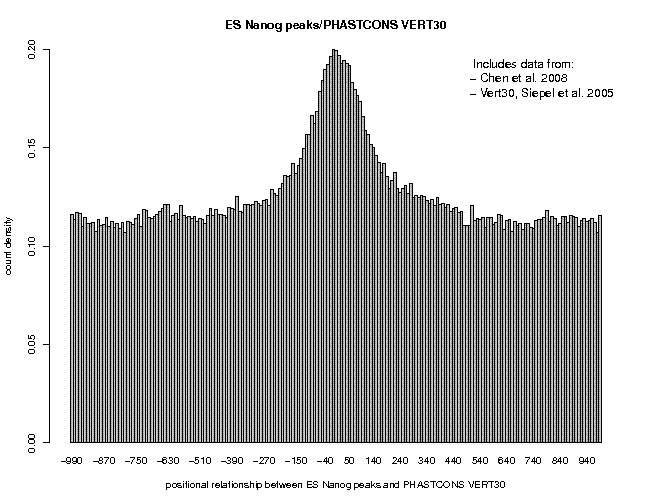
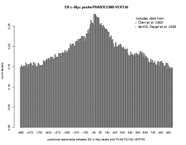
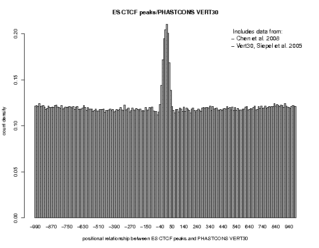
We see broad peaks for Nanog and c-Myc and a narrow peak for CTCF. This may indicate that the former two factors bind to target sites which are part of large cis-regulatory modules containing several conserved elements, whereas CTCF binds to isolated sites acting as stand-alone elements.
3. Correlation between site occupancy and cross-genome conservation
Background: Many transcription factors recognize short motifs that occur in very large numbers in a mammalian genome. Most of these potential binding sites are actually not occupied by the corresponding factor. One would naturally expect that the occupied sites are better conserved than the non-occupied sites. The following example illustrates how this question can be approached with a combination of tools from the ChIP-Seq and SSA servers.Step-by-step procedure: To proceed in this exercise you need the ES_nanog_peaks.fps files that has been generated in the tutorial Part A section 3. You can get it from your working directory or you can download it from here:
Go to the SSA server at: Choose FindM from the main menu and fill out the input form as follows:
SSA Input Data                           Signal Description

  x Upload FPS File                        x consensus: CCATCA
                                           Name: CCATCA
  ES_Nanog_peaks.fps                       Reference position: 3
  FPS name: From GEO
                                           Cut-off value:
Sequence Range                             x mismatches: 0

  5'border: -9999  3'border: 10000       Sequence Output

Sequence Selection and Search Criteria     Retrieve sequences in x FPS
                                           Sequence extraction range
  Search mode: bidirectional               (leave both fields blank)
  Selection mode: multiple non-
                  overlapping matches
|
Use the link "Save FPS File" to save the output file under the name Nanog_CCATCA.fps. The file can be found here:
We have extracted Nanog binding site motifs in a large area around in vivo bound Nanog sites. Therefore the resulting set of motif matches should contain bound as well as unbound sites. We are going to split this set into corresponding subsets using ChIP-cor with the following specifications:
Reference Feature: Target Feature: x Upload custom Data x Select available Data Sets Input format: FPS Genome: M. musculus (July 2007.. From file: .../ Nanog_CCATCA.fps Data Type: ChIP-Seq Sort input: on Series: Chen 2010, ES cells, ... Experiment: (default) Sample: ES Nanog Feature: (blank) Genomes: M. musculus (NCBI37/mm9) Additional Input Data Options: Strand: oriented Strand: any Centering: (blank) Centering: 65 Repeat Masker: unchecked Repeat Masker: unchecked Analysis parameters: Input Range : -1000 to 1000 Window width: 10 Count Cut-off value: 1 Normalization: count density |
This was just a preparatory step. We are now using the menu below under the header "Enriched Feature Extraction Option" to select those motif matches which have elevated Nanog ChIP-Seq tags in ES cells. Select the following parameters:
From -122 To: 122
Threshold: 15
Cut-Off: 1
Switch to Depleted Feature Extraction: off
Ref Feature Oriented: on
x Genomes: M. musculus (July 2007)
This retrieves 2079 occupied Nanog motifs. Save the output SGA file as Nanog_CCATCA_bound.sga. Now go back the the previous page and repeat the same procedure with the following parameter changes:
Threshold: 1
Switch to Depleted Feature Extraction: on
This extracts 42496 unbound sites. Save the output under the name Nanog_CCATCA_unbound.sga. The two resulting files can be found here. Now generate conservation profiles for these two files as explained in Section 6. The results are shown below.
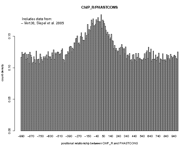
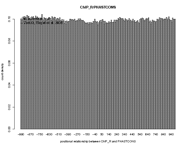
As you can see, the conservation profile for unbound motifs is flat. The conservation profile for bound motifs is somewhat broader than the one seen for all ChIP-Seq defined Nanog sites (Section 6), suggesting that Nanog-motif-containing binding sites differ somewhat from octamer-motif-containing and other binding sites.

