ChIP-Seq Analysis TutorialPart 1: ChIP-Seq Data Analysis
|
|
In this section, we will be giving a detailed example on:
A. Locating in vivo STAT1-binding sites
Methodology
A typical workflow for finding the most likely binding sites involves the following steps:
- Perform correlation studies by means of ChIP-Cor to estimate the average fragment length of the ChIP-Seq data under study, and to estimate the average background count density.
ChIP-Cor generates a positional correlation plot for two features that may be '+' and '-' strand tags from the same experiment:
- 5'-3' tag correlation is used for fragment length estimation and consequently for tag centering;
- autocorrelation analysis reveals the density of peaks that represent binding compare to the average background density. The average background density is then used to estimate a reasonable threshold for binding peaks.
- Shift tags mapping to the + or - strand towards the expected center of the DNA fragment by ChIP-Center to generate a SGA file containing centered tags. The shif amount is half the average fragment lenght.
- Find putative binding peaks by ChIP-Peak using the centered ChIP-Seq tags.
- We use regions of the genomes with low density reads as estimated background (ChIP-Cor).
- ChIP-Peak determines a cumulative tag count in a specified window of width w (in bp).
- The peak threshold parameter defines a minimal cumulative tag count for 'good' peaks, and is related to the
average background density by the following empirical formula:
Peak threshold = (bg density) x (w) x (fold enrichment)
where the 'fold enrichment' parameter is a sort of fold ratio that estimates enrichment relative to the background data (default value = 5).
1. 5'-3' Correlation (ChIP-Cor)
As a preprocessing step, we need to estimate the average fragment width of our
STAT1 ChIP-seq tags in order to find the most likely binding sites.
Each ChIP-DNA fragment has been sequenced and subsequently mapped to the
human genome (release NCBI36). The SGA file we work with contains a large
(approx 15 millions) set of start coordinates of sequence reads in both DNA strands.
We remind that sequences technologies preserve the strand specificity.
The relative distribution of 5'-3' start positions gives us an estimate of the average DNA fragment size that has been selected by ChIP.
A second preprocessing task is the background estimation in order
to safely identify peaks (or enriched regions) that represent real
binding sites.
The tool to perform these tasks on our ChIP-Seq Web server is
ChIP-Cor
(ChIP-Cor stays for ChIP-Seq Correlation tool).
Follow the instructions below:
|
You are now ready to submit the job.
As you can see, there are a number of parameters you can play with in order to make a graphically appealing correlation histogram.
- Change the window size and/or the count cut-off value.
- Look at a larger range, for instance -5000 to 5000, or at range:-400,+600 (which is centered around the peak).
As a post-processing step, ChIP-Cor on the Web performs non-linear curve fitting in the R environment useful for choosing parameters for peak finding. We assume that the best funtional form to model the correlation data is the Standard Normal Distribution whose probability density function having mean μ and standard deviation σ is given by the following formula:
|
We therefore try to fit the gaussian model to the correlation data around the main peak, using the workhorse nls function and making a starting guess for the mean value (μ) and the standard deviation(σ).
We use the predict method to find the function values for the fitted exponential function along the data interval around the main peak, and use these to plot the fitted gaussian function against the known correlation curve. The goodness-of-fit is summarized by the value of "residual" given as a result of the fitting function.
When applicable, we use the mean value of the gaussian function as an estimate of the average fragment size.
The results of the gaussian fitting are shown on the result page of ChIP-Cor under the header Statistics and Peak Finding Parameters Estimate. Below are the results for STAT1:
Gaussian Fit
Where we can see that the average fragment length of the STAT1 fragments is 150 bp, in agreement with previous observations.
Fit Parameters
In a typical peak finding application, one would first guess the centering distance by 3'-5' end correlation. Then one would use ChIP-cor again for an autocorrelation analysis with centered ChIP-Seq tags to estimate parameters for peak finding.
Go to ChIP-Cor and follow the instructions below:
|
The distribution is centered around 0 as expected, the peak is aprox 0.03 high, while the background density is 0.008, twice the previous value for the background density: this is because we are correlating data from a single source. The spread of the distribution (width) is approximately 300-400 bp.
As previously said, ChIP-Cor on the Web performs some downstream peak fitting calculations in order to help choose adequate paramenters for peak finding.
Given the following formula of the Gaussian fit:
|
The 'signal-to-noise-ratio' can be computed as follows:
s2n = b / (2 * a * σ)The term (2*a*σ) corresponds to the expected number of background counts under the peak area.
The expected number of random peaks discovered at different thresholds could be computed as follows
(for hg18):
window = 2 * σ genome_size = 3080315627 min = qpois(1 - c(30000)/genome_size * window, a * window) max = qpois(1 - c(100)/genome_size * window, a * window) nrd = (1 - ppois(seq(min,max,1), a * window)) * genome_size/windowThe value genome_size/window reflects the approximate number of tests carried out during a genome scan. We assume that counts in a window are Poisson distributed. We first determine low (min) and high (max) peak thresholds using the R poisson function which returns counts for given quantiles. Then we compute the expected number of peaks for all peak thresholds within the interesting range seq(min, max, 1). These values are displayed in the output page.
Listed below are the results for STAT1:
   Gaussian Fit

   Fit Parameters
For peak fitting, we recommend using a minimal window size of 10 (histogram bin) in ChIP-Cor.
For comparison, you can look at the correlation plot of CTCF, which is a major protein involved in insulator activity. Binding of targeting sequence elements by CTCF can block the interaction between enhancers and promoters, therefore limiting the activity of enhancers to certain functional domains. Besides acting as enhancer blocking, CTCF can also act as a chromatin barrier by preventing the spread of heterochromatin structures. In 2007, a ChIP-seq experiment (Barski et al.) generated high-resolution maps for the genome-wide distribution of 20 histone lysine and arginine methylations as well as histone variant H2A.Z, RNA polymerase II, and the insulator binding protein CTCF across the human genome using the Solexa 1G sequencing technology. These data are available on our Web server and they show a different fragment size distribution, indicating higher quality data. To confirm these claims:
- Produce a correlation plot for CTCF (Barski 2007)
- Analyse the fragment width distribution
- Estimate background density and peak count scoring
2. Peak identification (ChIP-Peak)
So far, we have used the ChIP-Cor tool to estimate the average fragment length of our STAT1 sequence reads (150 bp) as well as to provide clues for choosing the main parameter for both the peak and the partitioning algorithms: the peak count threshold in order to select 'true' STAT1 peaks. The main goal of ChIP-peak is to identify peaks corresponding to- have cumulative tag count ≥ Threshold
t - are local maximum with range ±
v/2
Optionally, the program performs refinement of peak centers (computes the center of gravity within window
As mentioned before, given our background distribution and the spread of the auto-correlation distribution of centered sequenced tags, we can reasonably choose a peak count Threshold t of 15 counts, and a peak window width w of 200 bp. In other words, good candidate peaks are enriched regions whose count score is greater than 15 counts. Our peak recognition algorithm is based on the assumption of a uniform background distribution. To extract STAT1 peaks go to the program ChIP-Peak (ChIP-Peak stays for ChIP-Seq Peak Identification tool) and procede as follows:
|
ChIP-Peak reports a total of 30735 putative STAT1 peaks.
You can try to extract peaks using different peak thresholds and compare the results.
The ChIP-Peak Web tool returns results in various output formats: SGA, WIG (for viewing the results on a Genome browser), and FPS. We mentioned before that FPS is a format specific to the Signal Search Analysis tools (SSA) to analyse sequence motifs that occur at characteristic distances upstream or downstream from a functional site in a nucleic acid sequence. We are going to use SSA later on to study the distribution of the TTCNNNGAA consensus sequence around the STAT1 peaks.
The WIG file can be uploaded to the UCSC genome browser via a direct link from the ChIP-Peak result page. The UCSC Genome Viewer provides a way to examine the data from a large number of genome assemblies, with extensive annotation tracks for various data types including known genes, predicted genes, mRNA and EST data, SNPs, comparative multi-species analysis and much more.
It also offers a way to manage and display custom traks either via the 'manage custom tracks' button on the Genome Browser page or by providing a specific URL.
As an example for STAT1 peaks found by ChIP-Peak, we show here the UCSC display of one particular STAT1 peak that co-localizes with a literature-derived STAT1 binding site recorded in the ORegAnno database:
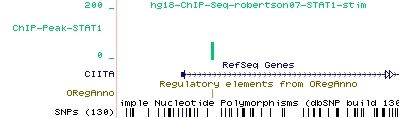
|
In Figure 1, the green vertical bar of the STAT1 track corresponds to a peak found by ChIP-Peak. Also shown is a corresponding STAT1 site from the ORegAnno track provided by the UCSC genome browser by simply turning on the ORegAnno 'Regulation Track'.
ChIP-peak also provides a Sequence Extraction option to extract sequences around peak centers in FASTA format. As we will soon see, this option is useful for downsteam analysis.
Before proceeding to motif analyis, we would like to refine our peak detection results by re-scoring the STAT1 peak list using the ChIP-Cor tool.
In order to do that:
- Save both the SGA and FPS files generated by ChIP-Peak.
   stat1_th15.sga

   stat1_th15.fps
3. Re-scoring Peak Centers (Optional)
This section is optional, it describes an alternative way to check for signal enrichment within detected peaks using ChIP-Cor together with the Feature Extraction application (also called ChIP-Score).
In the example studied so far, we already had some ideas on how to
identify STAT1 targets. We should keep in mind that identifying enriched
regions in target data by estimating a count fold-change based on tag count
distributions and a uniform background model is a challenging task.
Estimating whether a putative target site is a real binding site it is
not a simple binary decision-making process, in that there are many factors (such as DNA polymerase activity, changes in chromatin structure, sequence specificity, and others) that might modulate the
We would now like to check for STAT1 binding-sites enrichment within the extracted peaks using the ChIP-Cor tool.
We have so far used ChIP-Cor for correlating tag counts in opposite strands so as to get an estimate of the average sequence read width.
The ChIP-Cor program is in general applicable to other types of features
(e.g. TSS positions, histone modification sites, peak centers, etc.) as
it computes the relative correlation distance between two features by
producing a histogram indicating the frequency (in counts) of the target
feature as a function of the relative distance to the reference feature.
The frequency can be normalized to represent a density count frequency
(target feature counts/bp) or just a count fold-change of the target feature
with respect to the reference feature (global normalization).
If we therefore correlate STAT1 candidate peaks with centered STAT1 tags we should find enrichment at the peak centers, namely at 0.
Let us see if this is so.
Go to the program ChIP-Cor and do the following:
|
As expected, the distribution is peaked around n=0, meaning that our previously extracted peaks are enriched in STAT1 signals.
Further suggestion:
|
Have a look at the re-scored peak centers: the Feature Extraction Web tool generates both an SGA and FPS file representing the enriched peaks. One can also extract the sequences around the peak centers in FASTA format. We will use this feature later on for finding the STAT1 binding site motif with the MEME program.
We would now like to study motif enrichment in the peak regions that we have just extracted. We already know that most of the STAT1 binding sites contain the consensus sequence TTCNNNGAA. If the peaks found by ChIP-Peak indeed correspond to real binding sites, one would expect to find this motif in the vicinity of the extracted peak center positions. To test this assumption, we are going to use the program OProf from the SSA Web server. We will do this in the next Paragraph.
Note that the total number of peak center positions extracted by re-scoring the peak counts is lower (7625) than the total number of peaks (30735) previously reported by ChIP-Peak. This is because we have applied a more stringent peak threshold to re-score the peak regions.
Alternatively, we could have used the ChIP-Peak tool with a threshold of 30 tags per window.
4. Studying motif enrichment around peak regions
The program OProf (for Occurrence Profile) is used to analyse the distribution or location of a known motif relative to some specific functional sites. In our example, we know that a sizeable fraction of STAT1 binding sites contain the TTCnnnGAA consensus motif. We are therefore interested in studying the occurence of the STAT1 motif at relative distances from the STAT1 peak centers previously identified in a sliding window of 100 bp.Go to the OProf page and follow the instructions below:
|
You are now ready to submit the job.
As you can see, there are a number of parameters you can play with in order to make a graphically appealing signal occurrence profile.
- Change the window size and/or the number of mismatches allowed.
- Look at a smaller range, for instance -99 to 100.
5. Analysing the contents of peak regions
In the example studied so far, we already had some idea of how the motif we were interested looked like. But how to proceed if we know absolutely nothing in the beginning. In such cases, the program SList (for Signal List) can be of some help. SList is used to analyse the contents of signal-rich regions: it produces a list of locally over- or under-represented "signals" (oligonucleotide motifs).We will use SList to find motifs within STAT1 peak regions.
|
SList will produce a list of sorted by st-dv pentamer sequences (4 out 5 matches) that are locally over-represented within the scanned windows across the whole set of input sequences. In our case, input sequences represent STAT1 peak centers, so SList extracts 1000 bp long sequences which are centered around those peak centers. We are primarily interested in consensus sequence motifs that are over-represented within these regions.
Here is a partial list of top-ranked signals found by SList:
# Pos.    Signal           Frequency  st-dev
#
    0.50  CGGAA             0.8366   28.4830
    0.50  TTCCG             0.8341   27.6000
   10.50  CCGGA             0.7637   23.8740
   10.50  TCCGG             0.7618   23.6360
   -9.50  TCCGG             0.7595   23.2330
   10.50  CGGGA             0.7821   22.3110
    0.50  CCGGG             0.7193   21.1410
    0.50  TCCCG             0.7715   20.7630
   10.50  CCCGG             0.7124   20.5810
   10.50  GGAAA             0.8936   19.4320
   -9.50  TTTCC             0.8900   18.8050
   10.50  GGAAG             0.8850   18.3110
   20.50  GGAAC             0.8602   18.0500
   -9.50  GTTCC             0.8598   17.7810
    0.50  CTTCC             0.8844   17.7120
   10.50  GGGAA             0.8584   16.6160
   -9.50  GGGAA             0.8568   16.2850
    0.50  TTCCC             0.8560   16.2520

....
The position (Pos.) of the over-represented pentamers refers to the position (in bp) of the center of the sliding window with respect to the center of the input sequences (that is the peak center). We notice that the top-ranked words all conform to the consensus sequence TTCNNNGAA :
....CGGAA
TTCCG....
...CCGGA.
.TCCGG...
...CGGGA.

TTCCSGGAA
Such overlaps are often seen in word lists returned by SList.
6. Optimizing a weight matrix for the STAT1 sequence motif
Consensus sequences are not always appropriate descriptors of regulatory sequence motifs. In particular, they cannot make a difference between easily tolerated and severe mismatches. Note that a weight matrix can be viewed as a generalization of a consensus sequence.In this section we will try to find an optimal weight matrix description for the STAT1 motif. The program PatOp (for Pattern Optimization) implements an iterative procedure which successively optimizes the weight matrix, the cut-off value, and the borders of the preferred region of occurrence, keeping two of these three components constant at a time. PatOp has the capability of extending the matrix to the left and right side if additional consensus is observed, or to drop positions in the opposite case. PatOp uses a heuristic algorithm converging to a local optimum.
We will use PatOp to produce a weight matrix description of the STAT1 motif.
Start from the consensus sequence motif TTCNNNGAA (one mismatch).
Like with OProf:
|
The optimized matrix for the STAT1 sequence motif as defined by our ChIP-Seq data is the following:
    Weigth Matrix

    Sequence Logo


-1.12   -0.61   -1.15    0.00
-4.67   -3.70   -4.75    0.00
-4.37   -4.49   -2.82    0.00
-2.09    0.00   -4.21   -3.48
-3.11    0.00   -4.04   -1.07
 0.00   -0.21   -0.24   -0.02
-1.05   -4.37    0.00   -3.13
-3.15   -4.13    0.00   -2.04
 0.00   -2.74   -4.21   -4.28
 0.00   -4.80   -3.83   -4.79
 0.00   -1.24   -0.60   -1.07


  CO    82.00% (cut-off value  -7.09)
You can now try to use OProf to analyse the occurence profile of the optimized STAT1 motif around our identified peak regions (use both stat1_th15.fps and stat1_th30.fps for comparison).
Hint: under Cut-off value activate the checkbox absolute and fill in value -7.09.
7. Motif discovery in high-scoring peak regions
As we have seen in the previous Paragraphs, consensus sequences can only approximately describe the binding specificity of a transcription factor, and in addition the DNA-binding domain of a protein under study may not be known in advance. That is the reason why we may want to apply an ab initio motif discovery algorithm such as MEME or RSAT to a set of putative peak regions.Both MEME and RSAT are suitable and reliable tools for de novo detection of regualtory elements, the advantage of RSAT being that it supports a larger number of sequences.
We first apply MEME to the STAT1 peak regions found by ChIP-Peak. MEME uses a motif-based search strategy to scan a group of DNA or protein sequences.
Since MEME can only process a limited amount of DNA sequence data in a limited amount of time, we repeat the peak finding step with a high count threshold of 200 counts per window. We run ChIP-Peak as in Paragraph 2, changing the following:
- Extract peaks with a threshold of 200.
- Activate Repeat Masker to filter out interspersed repeats and low complexity DNA regions.
The output page of ChIP-Peak includes a Web form that allows users to extract DNA sequences in Fasta format within an adjustable range relative to the peak center positions.
Use the Sequence Extraction tool with the following parameters:
- range: -65; 65 bp.
You end up with the following sequence files for the MEME analysis:
   stat1_th200_RM.seq  (265 peak regions)
   stat1_th200_noRM.seq (350 peak regions)
Go to the MEME Server and proceed as follows:
- Enter your e-mail address
- Upload the Fasta-formatted sequence file extracted with ChIP-Peak
- Choose 50 as the Minimum optimum number of sites for each motif.
- Set as Minimum and Maximum width of your motif the value 12.
- Keep the other MEME parameters at their default values.
You can also run the MEME program using the default parameters.
You are going to wait a while to get the results. You will promptly receive an e-mail with information about your job submission, and a link to the MEME result page.
Here are the results from MEME in HTML format with and without prior repeat masking:
- MEME HTML Results ; MEME HTML Results (def) (Repeat masking)
- MEME HTML Results ; MEME HTML Results (def) (no Repeat Masking)
As we can see from the MEME results, about 97-98% of all STAT1 sites in both datasets contain the full 9-bp consensus STAT1 motif:
Note that without repeat masking, MEME finds two other motifs contained in about 4% of STAT1 sites:


These two motifs are part of the MER41B sequence, a rare LTR repetitive element of the human genome, as it is depicted in the figure here below:
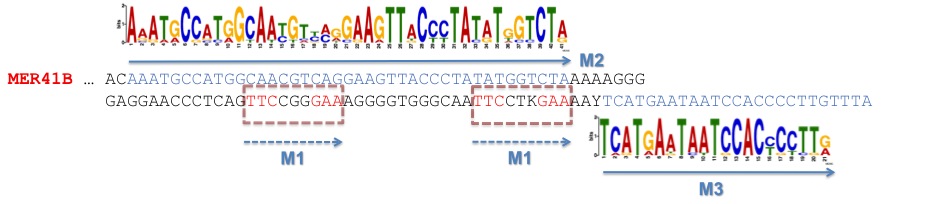
Figure 2. Consensus binding motifs for STAT1 binding sites found by MEME are part of the MER41B sequence.
The figure shows a portion of the MER41B consensus sequence from the Repbase collection.
Another group (Jothi et al., Nucleic Acids Res. 36:5221) has identified two different motifs in the same STAT1 dataset (Robertson et al.):
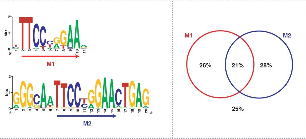
Figure 3. Accuracy of inferred binding sites. Jothi et al.
Consensus binding motifs for STAT1 binding sites are shown on the left panel. The right panel shows the percentage of identified binding sites containing the consensus binding motif(s).
In the case of STAT1, 75% of all binding sites contained the classic GAS motif TTC(T/C)N(G/A)GAA. About 54% of all STAT1 sites contained either the M1 or the M2 motif (Figure 2), while 21% of all STAT1 sites contained both M1 and M2.
It has been found that:
- A rare LTR repetitive element (MER41B) contains STAT1 motif pairs at a relative distance of 21 bp: it is a combination of both M1 and M2 motifs;
- Most STAT1 motif pairs with 21 bp distance come from MER41B retro-elements;
- Most of the STAT1 site pairs in MER41B are occupied in vivo;
- MER41B explains motif M2 found by Jothi et al. (2008);
- A sizable fraction (>5%) of in vivo STAT1 sites reside in MER41B retro-elements.
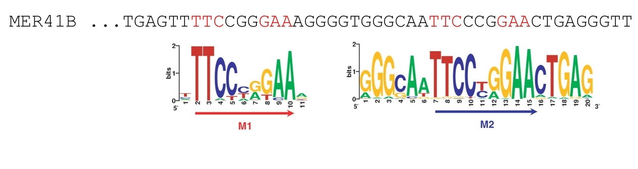
Figure 4. STAT1 motif pairs (M1-M2) in MER41B.
Take-home lesson : Exclude peaks in repeat regions for motif discovery!
We now use the RSAT-tools pipeline for discovering motifs in the STAT1 peak sequences.
For that, we first extract fasta sequences within the range [-100;100] around STAT1 peak centers with threshold 50 using the same procedure as described above. The sequence file is the following:
stat1_th50_+-100.seq (2400 peak regions)
Go to the RSAT Server and proceed as follows:
- Select the peak-motifs analysis tool under NGS - ChIP-seq
- Upload the Fasta-formatted sequence file extracted with ChIP-Peak
- Select the checkbox Discover words with local over-representation under Motif discovery parameters.
- Keep the other RSAT-tool parameters at their default values
- Enter your e-mail address
Here is the result page form RSA-tools - peak-motifs:
As we can see from the RSAT results, the main motif corresponds to canonical STAT1 motif:
8. Genomic annotation of ChIP-seq peaks
For peak annotation, we recommend using Nebula, which is a web service provided by Institut Curie and powered by Galaxy for ChIP-seq data analysis, or GREAT from Bejerano Lab at Stanford, which is a tool aimed at predicting functions of cis-regualtory regions.
The GREAT Programming Interface allows external clients to submit BED data automatically for analysis by GREAT and display in the GREAT user interface. We provide a link to GREAT in the output page of ChIp-Peak.
Here below is an example of such data submission for the Robertson 2007 STAT1 set (Example).
The peak file in BED format is the following:
chip_peak_stat1_200_50.bed (3280 peak regions)To submit this data to GREAT, the client webpage includes a link that sends an HTTP GET request to GREAT. When the link is clicked, the request is sent to GREAT:
Link to GREAT
In order to use Nebula, go to the Nebula Web page, and proceed as follows:
- Upload the BED-formatted peak file generated with ChIP-Peak using the Get Data tool
- Select the Genomic annotation of ChIP-seq peaks analysis tool under NGS: Peak Annotation
- Select organism: Homo sapiens
- Select genome version: hg18
- Keep all other parameters unchanged
The results from Nebula appear within the History frame and are depicted in the figure here below:
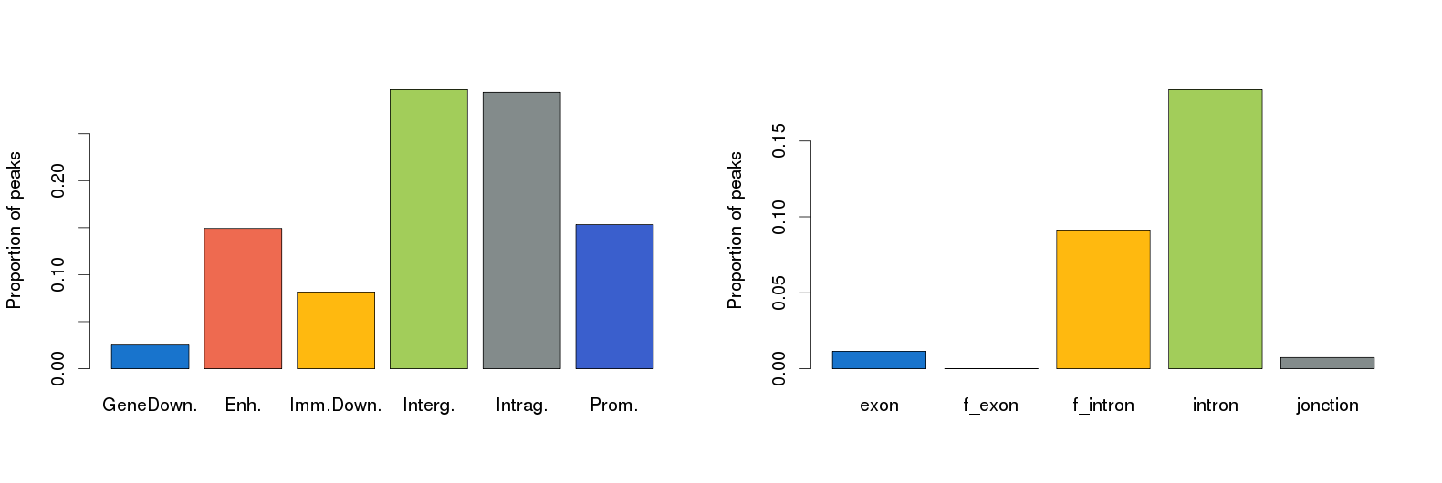
The Nebula tools generates other files in tabular format:
   Galaxy-Annotated_Peaks_ChIP-Peak-200-50.txt  (Peak location distribution)
   Galaxy-LOG_for_Annotated_Peaks_200-50.txt  (Log for annotated peaks)
The results are in agreement with what is reported in the literature (Robertson et al., Nat Methods. 2007 Aug;4(8):651-7).
9. Further Analysis
Of course, there are many more interesting biological questions that one could address using ChIP-Seq data in combination with other data types such as cross-genome conservation maps, promoter regions, and histone modification profiles:- Cross-genome conservation of in vivo occupied TF binding sites;
- Position of TF binding sites relative to transcription start sites;
- Position of transcription start sites relative to nucleosomes.
