Nucleosomes around TFBS

Chip-seq data analysis: from quality check to motif discovery and more

Lausanne, 27 March - 31 March 2017

Data reproduction exercise: Nucleosome organization around YY1 sites.

Author: Philipp Bucher

Introduction

This exercise is based on the following paper:

et al.

This paper contains many results covering diverse aspects of transcription factor binding sites. In this data reprroduction exercise, we focus on the part that deals with the nucleosome architectures, see results subsection:

The ChIP-seq peaks of many TFs are flanked by positioned nucleosomes

Specifically, we will try to reprocude results shown in Figure 5a and 5b.

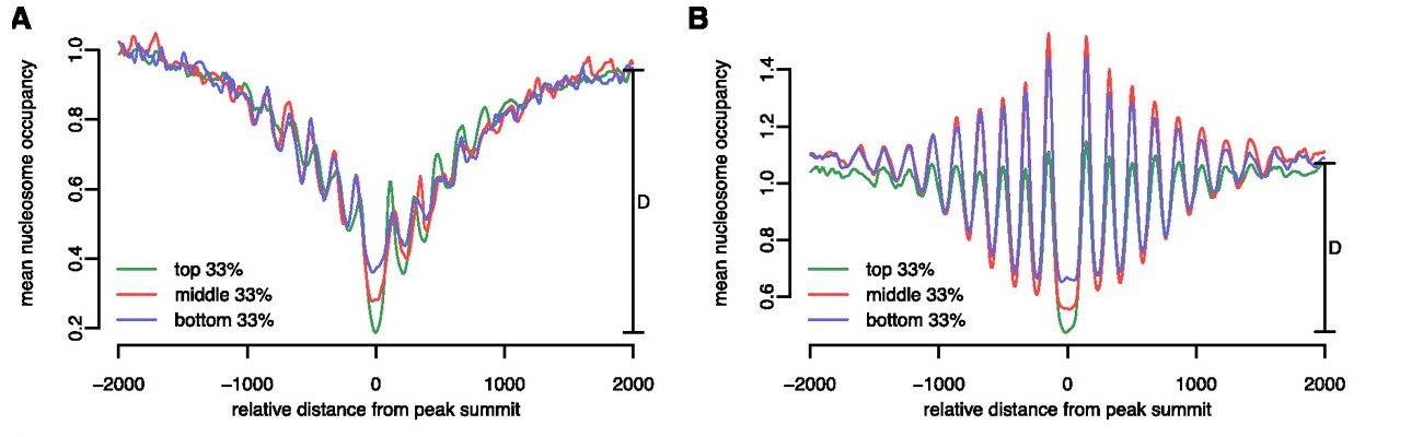
The Figure shows average nucleosome occupancy profiles around YY1 binding sites in the lymphoblastoid cell line GM12878. The peak lists were first divided into promoter-proximal and promoter-distal binding sites and further stratified into three groups based on ChIP-seq signal strength.

The authors of the paper describe and interpret the results as follows:

"We distinguish nucleosome occupancy and nucleosome positioning, with occupancy defined as the area under the occupancy profile and positioning defined as the regularity of the oscillatory pattern in the occupancy profile. Thus, the regions around TSS-proximal summits tend to show lower nucleosome occupancy and lower nucleosome positioning than regions around TSS-distal summits (cf. Fig. 5A,B). This difference may reflect the effects of RNA polymerase on chromatin structure (Weiner et al. 2010). Within the proximal and distal categories, the top, middle, and bottom third peaks, which correspond to the peaks with strongest, medium, and weakest TF binding, tended to show the greatest, medium, and weakest nucleosome positioning (Fig. 5A,B)."

Exercise

Try to reproduce the above Figure with public data available from the ChIP-Seq server

Hints and recipes

Input data from human genome assembly hg19

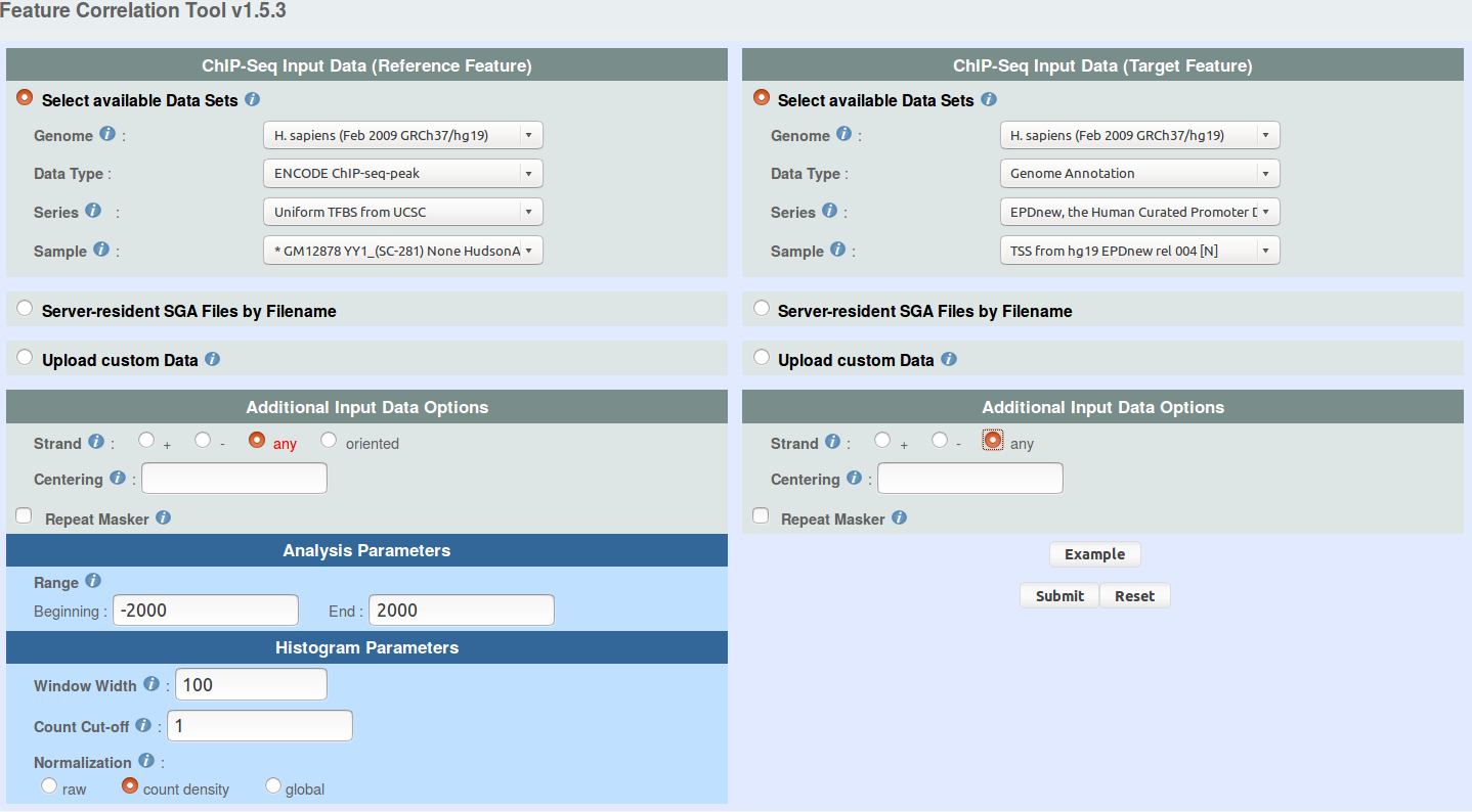
    ENCODE ChIP-seq-peak -> Uniform TFBS from UCSC 
       sample: GM12878 YY1_(SC-281) None HudsonAlpha peaks 
    ENCODE DNase FAIRE etc. -> GSE35586, Nucleosome Position by MNase-seq ...
       sample: Nucleosome Gm12878 rep1 
    Genome Annotation -> EPD, the Human Curated Promoter Database
       sample: TSS from hg19 EPDnew rel 003

Note: The MNase data files are very voluminous and thus take time to process (minutes rather than secons). We therefore recommend to generate the figures with one replicate only.

Making a nucleosome occupancy profile for distal YY1 sites.

In the paper, the authors write:

"We also divided the peaks for each TF into two sets, those within 2 kb of transcription start sites (TSS-proximal) and those >2 kb away from TSS (TSS-distal)."

Got to the ChIP-Cor input form. Select the above indicated YY1 peak list as reference feature and the TSS from EPDnew as target feature (other parameters are not important at this stage). On the results page use the "Enriched Feature Extraction Option" submenu to extract YY1 sites that do or do not have an annotated TSS within 2kb. (toggle "Depleted Feature Extraction" on/off). From the next page, navigate directly to ChIP-Cor using the action button near the lower right corner. Then run ChIP-Cor with the above indicated MNase sample as target feature (strand option "all", centering distance 70).

Stratifying the YY1 peaks into three subsets by signal strength

One way of doing this is by downloading the peak SGA file from the MGA repository via the MGA overview page at:

/chipseq/data/html/res_data.php

The name of the compressed SGA file is:

wgEncodeAwgTfbsHaibGm12878Yy1sc281Pcr1xUniPk.sga.gz

The 6th column of this extended SGA file contains a statistical binding site score which can be used for ranking. The three subsets can be generated in R are as follows:

sga=read.table("wgEncodeAwgTfbsHaibGm12878Yy1sc281Pcr1xUniPk.sga.gz", header=F)
dim(sga)
N=dim(sga)[1]

r1 = 1:floor(N/3)
r2 = (floor(N/3)+1):floor(2*N/3)
r3 = (floor(2*N/3)+1):N

bottom = sort(order(sga[,6])[r1])
middle = sort(order(sga[,6])[r2])
top    = sort(order(sga[,6])[r3])

write.table(sga[bottom,], "GM12878_YY1_bottom.sga",
   quote=F, sep="\t", row.names=F, col.names=F)
write.table(sga[middle,], "GM12878_YY1_middle_sga",
   quote=F, sep="\t", row.names=F, col.names=F)
write.table(sga[top,],    "GM12878_YY1_top.sga",
   quote=F, sep="\t", row.names=F, col.names=F)

You can now individually upload these SGA files to the ChIP-cor server and repeat the previously outlined procedure to generate nucleosome occupancy plots.

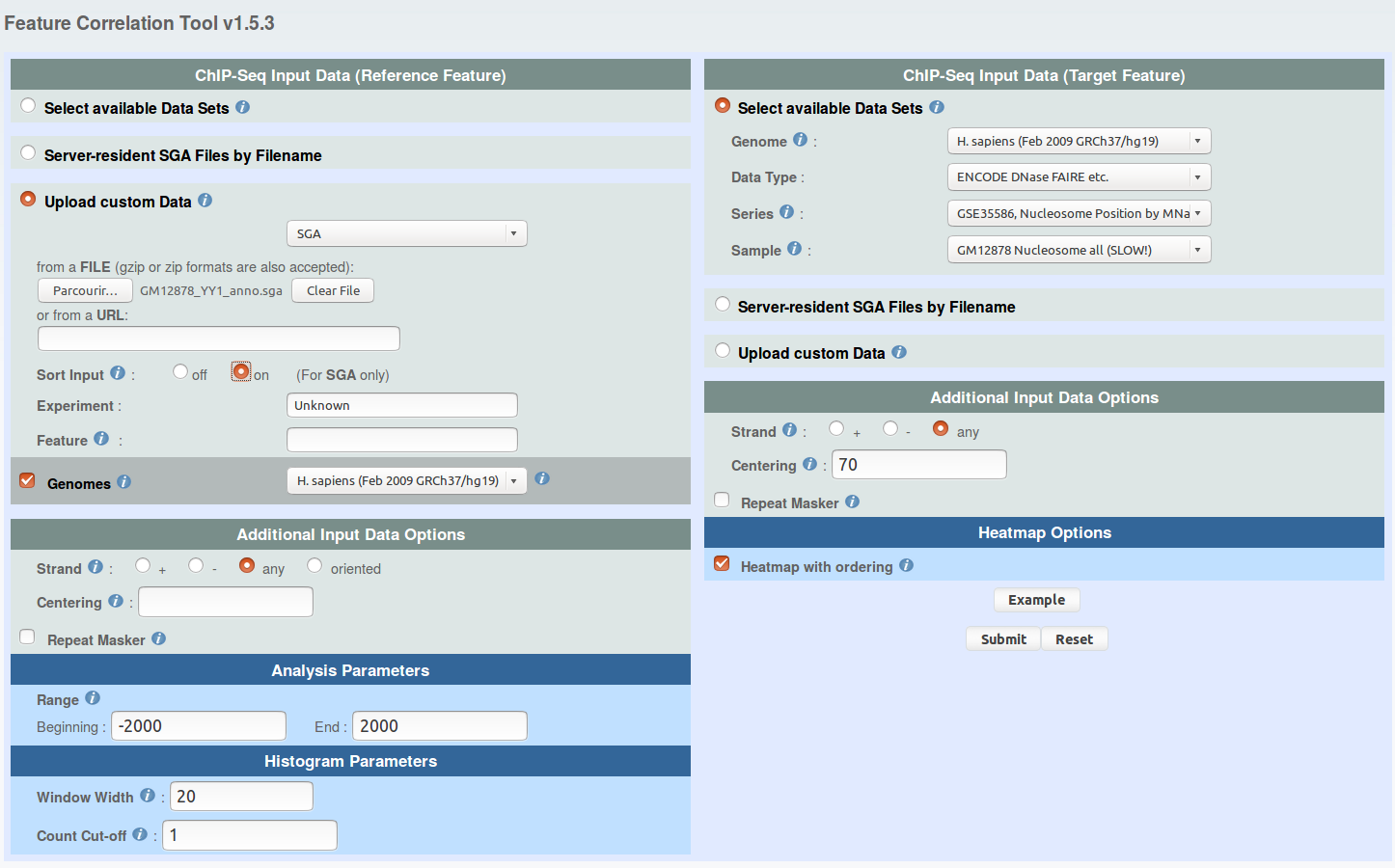
A more efficient prodedures to reproduc Figures 5a and 5b at once

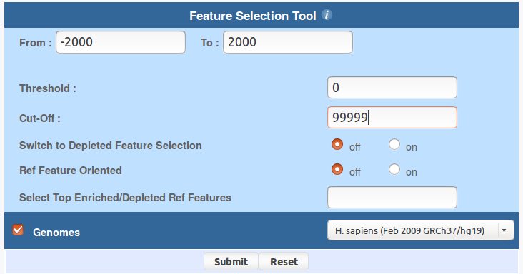
You can use ChIP-Cor to generate an extended YY1 peak file with promoter status annotation. Select the above indicated YY1 peak as reference feature and EPD promoters as target feature. Have a look at the following pictures to set the parameters. In essence, the use of the "Enriched Feature Extraction Option" with Threshold=0 will result in selecting all the promoters. However, you will know the number of TSS beside every peak. Save the resulting SGA file under the name GM12878_YY1_anno.sga (or get it here).

This is an extended SGA files with peak scores in the 6th field and the TSS counts in the 7th field as shown below:

NC_000001.10   YY1_P   714001	0   1   133.535942201664   0
NC_000001.10   YY1_P   805331	0   1   46.6896250548417   0
NC_000001.10   YY1_P   840144   0   1	70.0879017887289   0
NC_000001.10   YY1_P   894612   0   1	244.724808404057   2
NC_000001.10   YY1_P   895930   0   1	40.8279820108751   2

You can now upload this file to the ChIP-Extract input form at:

/chipseq/chip_extract.php

in order to extract the nucleosome occupancy data. Set the parameters as displayed below. This will be slow - it will take about 20 mins. However once you have the output files, you can do everything that in R very rapidly.

From the ChIP-Extract results page, download the "Ref SGA File" and the "Table (TEXT)" under the names:

GM12878_YY1_anno.sga

GM12878_YY1_nucl.txt

Actually, it is not necessary to save the SGA file again since it is identical to the uploaded file. However, it is good practice to always save the two files together, in order to be sure that the sorting of the reference features is the same in the data and in the annotation file.

Below is the R recipe to generate the plots equivalent to Figure 5a and 5b in the paper.



	# data input, defining the proximal and distal peak subsets
	anno=read.table("GM12878_YY1_anno.sga")
	data=as.matrix(read.table("GM12878_YY1_nucl.txt"))
	prox=which(anno[,7] != 0)
	dist=which(anno[,7] == 0)

	# top, middle, bottom subsets for proximal and distal peaks
	N           = length(prox)
	r1          = 1:floor(N/3)
	r2          = (floor(N/3)+1):floor(2*N/3)
	r3          = (floor(2*N/3)+1):N
	prox_bottom = prox[sort(order(anno[prox,6])[r1])]
	prox_middle = prox[sort(order(anno[prox,6])[r2])]
	prox_top    = prox[sort(order(anno[prox,6])[r3])]

	N           = length(dist)
	r1          = 1:floor(N/3)
	r2          = (floor(N/3)+1):floor(2*N/3)
	r3          = (floor(2*N/3)+1):N
	dist_bottom = dist[sort(order(anno[dist,6])[r1])]
	dist_middle = dist[sort(order(anno[dist,6])[r2])]
	dist_top    = dist[sort(order(anno[dist,6])[r3])]

	layout(matrix(1:2, nrow=1, ncol=2))

	# plotting Figure 5a
	x = 20*(-99:99); par(cex=1.2)
	plot(x,colMeans(data[prox_top,]),t="l", col="green", ylim=c(1.5,6),
	     xlab="relative distance to peak summit",
	     ylab="mean nucleosome occupancy")
	par(new=T)
	plot(x,colMeans(data[prox_middle,]),t="l", col="red", ylim=c(1.5,6),
	     xaxt="n", yaxt="n", xlab="", ylab="")
	par(new=T)
	plot(x,colMeans(data[prox_bottom,]),t="l", col="blue",  ylim=c(1.5,6),
	     xaxt="n", yaxt="n", xlab="", ylab="")
	legend("bottomleft", legend=c("top 33%","middle 33%", "bottom 33%"),
	       lty=1, col=c("green","red", "blue"), bty="n")

	# plotting Figure 5b
	x = 20*(-99:99); par(cex=1.2)
	plot(x,colMeans(data[dist_top,]),t="l", col="green", ylim=c(4,7.5),
	     xlab="relative distance to peak summit",
	     ylab="mean nucleosome occupancy")
	par(new=T)
	plot(x,colMeans(data[dist_middle,]),t="l", col="red", ylim=c(4,7.5),
	     xaxt="n", yaxt="n", xlab="", ylab="")
	par(new=T)
	plot(x,colMeans(data[dist_bottom,]),t="l", col="blue",  ylim=c(4,7.5),
	     xaxt="n", yaxt="n", xlab="", ylab="")
	legend("bottomleft", legend=c("top 33%","middle 33%", "bottom 33%"),
	       lty=1, col=c("green","red", "blue"), bty="n")