Model definition and data generation: R script Hide script

Composite peak data

K=2; L=63; r=list(1:21,22:42,43:63)
C=matrix(nrow=K, ncol=sum(L))
C[1,r[[1]]] = 2*dnorm(1:21, 8,1.0)
C[1,r[[2]]] = 5*dnorm(1:21, 8,3.0)
C[1,r[[3]]] = 1*dnorm(1:21,11,0.5)
C[2,r[[1]]] = 4*dnorm(1:21, 8,3.0)
C[2,r[[2]]] = 3*dnorm(1:21,14,1.0)
C[2,r[[3]]] = 1*dnorm(1:21, 8,0.5)
Q = c(0.6,0.4)

Definition of random samples

N=10000
samples=matrix(data=0, nrow=N, ncol=K)
rs=sample(1:K,N,rep=T,prob=Q)
for(i in 1:N) {samples[i,rs[i]]=1}

Random data generation

data=matrix(nrow=N, ncol=L) 
for (i in 1:N) {data[i,] = rpois(L,C[which(samples[i,] == 1),])}

# Let's have a look at the aggregation plot of the complete set
plot(colMeans(data), type = "l")

Various partitioning methods: R script Hide script

Load the em_functions.R file:

source("em_functions.R")

Partioning with random seeds

c=matrix(nrow=L, ncol=K)
  p=matrix(nrow=N, ncol=K)
  for(i in 1:K) {p[,i] = rbeta(N,N**-0.5,1)}
  c = (t(p) %*% data)/colSums(p)
  q=rep(1/K,K)
  for(i in 1:20) {em_shape(c,q,data); plot_classes(c); print(q)}

Iterative partitioning

c    = matrix(data=colMeans(data), nrow=1, ncol=L)
  flat  =matrix(data=    mean(data), nrow=1, ncol=L)
  q = 1

  for (m in 1:(K-1)) {
     c = rbind(flat,c)
     q = c(1/m,q); q = q/sum(q)
     for(i in 1:20) {em_shape(c,q,data); plot_classes(c); print(q)}
     }

Iterative partitioning with untrained flat class

c    = matrix(data=colMeans(data), nrow=1, ncol=L)
  flat  =matrix(data=    mean(data), nrow=1, ncol=L)
  q = 1
  for (m in 1:(K)) {
     c = rbind(flat,c)
     q = c(1/m,q); q = q/sum(q)
     for(i in 1:20) {
        c[1,]=flat; em_shape(c,q,data); plot_classes(c); print(q)}
     }

Model evaluation: R script Hide script

cor(p, samples) # Pearson's correlation between the real and predicted class probabilities

Part II: CTCF dataset [GEO series GSE29611 Histone Modifications by ChIP-seq from ENCODE/Broad Institute]

In the current exercise we will be trying to reproduce one of the figures from following paper:

Nair et al., 2014, Probabilistic partitioning methods to find significant patterns in ChIP-Seq data, Bioinformatics, 30, 2406-2013, PMID 24812341



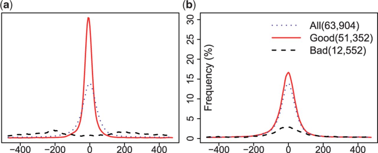
Shape-based peak evaluation with shifting. The figure illustrates the effects of probabilistic partitioning on a CTCF peak list provided by ENCODE in terms of motif enrichment. (a) Probabilistic partitioning with shifting. (b) Partitioning based on original P-values.

In order to reproduce the above figure, we will need an ENCODE peak list and associated tags data.

• ENCODE peak list for CTCF from HUVEC cell line. Download the peak list.
• Process tags data from HUVEC cell line. We will use it directly from the server.

Pre-processing of data to generate tag count matrix.

We will use ChIP-Extract Analysis Module to generate a tag count matrix in defined bins around CTCF sites. Select appropriate target feature and then click submit.

• Reference feature: above peak list
• Target feature: hg19; ENCODE ChIP-seq; GSE29611; HUVEC CTCF (do appropriate centring)
• Analysis parameters: -500 to 500; Window width:10; Count cut-off:1

Download the Ref SGA File and Table (TEXT) and save as huvec_peaks.sga and huvec_ctcf.txt respectively.

Perform iterative shape based partitioning with shifting and prepare data for motif enrichment analysis. R script Hide script

Read data:

data = as.matrix(read.table("huvec_ctcf.txt"))

Define classes and shifts:

K=1; S=11; N=dim(data)[1]; L=dim(data)[2]-S+1; ITER=10 

Iterative shape based partitioning with shifting

c = colMeans(data[,(floor(S/2)+1):(floor(S/2)+L)])
flat = matrix(data=mean(data), nrow=1, ncol=L)
q=q0 = dnorm(1:S,floor(S/2)+1,1)/sum(dnorm(1:S,floor(S/2)+1,1))

  for (m in 1:(K)) {
     c = rbind(flat,c)
     q = rbind(q0/m,q); q/sum(q) 

     for(i in 1:ITER) {reg_shift(q); c[1,]=flat;
        reg_shift(q); em_shape_shift(c,q,data); plot_classes(c); print(q)}
	}
prob = rowSums(p[,2,])
shift = apply(p,c(1,3),sum) %*% (1:S)

Read peaks and filter based on probability value into different classes:

peak <- read.table("huvec_peaks.sga", header=F, sep="\t")
good <- peak[which(prob>=0.5),]
bad <- peak[which(prob<=0.5),]
peak[,3] <- round(peak[,3]+10*(shift-6))
good_shifted <- peak[which(prob>=0.5),] # good peaks after shifting

Write output as sga files.

write.table(good, "chipPart_good.sga", sep="\t", quote=F, row.names=F, col.names=F)
write.table(bad, "chipPart_bad.sga", sep="\t", quote=F, row.names=F, col.names=F)
write.table(good_shifted, "chipPart_good_shifted.sga", sep="\t", quote=F, row.names=F, col.names=F)

Read the bed file and sort based on p-value generated by ENCODE consortium. For fair comparison, the threshold for partitioning with the original p-values is chosen such as to match the numbers of good and bad peak obtained with probabilistic partitioning.

pval <- read.table("ctcf_peaks.bed", header=F, sep="\t")
spval <- pval[order(pval[,8], decreasing=T),]
goodpval <- spval[1:nrow(good),]
badpval <- spval[nrow(good)+1:nrow(pval),]
write.table(goodpval, "pval_good.bed", sep="\t", quote=F, row.names=F, col.names=F)
write.table(badpval, "pval_bad.bed", sep="\t", quote=F, row.names=F, col.names=F)

Use ChIP-Convert to convert the output of partitioning into following formats.

• bed to sga for p-value classes

Following piece of experiment needs to be carried out on SSA web-server. Extract CTCF motif enrichment (for all the sga files produced in previous step) using Oprof

• OProf Parameters: -499 to 500; Window size: 50, Window shift: 1; Search mode: bidirectional; Cut-off: p-val: 1.0000e-05
• PWM from library: JASPAR CORE 2014 vertebrates; Motif: CTCF MA0139.1 (length=19)

Save the graph output as: good_part.txt, bad_part.txt, good_shifted_part.txt, high_pvalue.txt, low_pvalue.txt and ctcf_all.txt (for all the sites)

Plot the results (as shown in above figure). Show plotting script Hide script

Now move back into R for plotting the results. This will produce the figure as shown above.

## read files that were the output/ graph text output from Oprof and plot results:
a <- read.table("good_part.txt", header=T, sep="")
b <- read.table("bad_part.txt", header=T, sep="")
c <- read.table("good_shifted_part.txt", header=T, sep="")
d <- read.table("high_pvalue.txt", header=T, sep="")
e <- read.table("low_pvalue.txt", header=T, sep="")
all <- read.table("ctcf_all.txt", header=T, sep="")

par(mar=c(0,2.75,1,1), mfrow = c(1,2), oma=c(4,0,2,0))
plot(c[,1],c[,2],type="l",lwd=2, col="red", cex.axis=1, xlab="", ylab="", yaxt="n", ylim=c(0,30));
points(c[,1],all[,2],type="l",lwd=2, col="blue", lty=4)
points(c[,1],b[,2],type="l",lwd=2, lty=3)
plot(d[,1],d[,2],type="l",lwd=2, col="red", cex.axis=1, xlab="", ylab="", ylim=c(0,30));
title(ylab="Frequency (%)", cex.lab=1, mgp=c(-2.2,2,1))
points(c[,1],all[,2],type="l",lwd=2, col="blue", lty=4)
points(c[,1],e[,2],type="l",lwd=2, lty=3)
legend("topright",c("All(63,904)","Good(51,136)","Bad(12,768)"),col=c("blue","red","black"), lwd=c(1,1,1), cex=1, box.col=NA, bty="n", lty=c(4,1,3), seg.len=2)

Part III: Nucleosome organization around transcription factor binding sites in GM12878 cells. For this exercise, the datasets come from the following sources : ENCODE Uniform, GSE32970, GSE35586, GSE29611

Here are the needed R functions em_api.R. Download this file and store it in the directory you will work in. The code below contains calls to these functions.

In this exercice, we will investigate the nucleosome organization around CTCF and ETS1 binding sites in GM12878 cells. CTCF is a factor which is known to show nicely phased nucleosomes arrays on each side of its binding sites. ETS1 is a transcription factor which is mostly found near transcription start sites (TSS) but which does not behave as CTCF regarding nucleosome organization.
We will first extract CTCF and ETS1 peaks from peak lists which have the corresponding factor motif in their neighbourhood using FindM. Then, we will measure the density of MNase and DNAseI reads around these peaks by generating matrices of tag counts using ChIP-Extract. We will import these data in R and perform a probabilistic partitioning to try to identify several nucleosomes organization classes around transcription factor binding sites and isolate classes of interest. Finally, we will extract one class of interest and go back to ChIP-Cor for additional analyses.

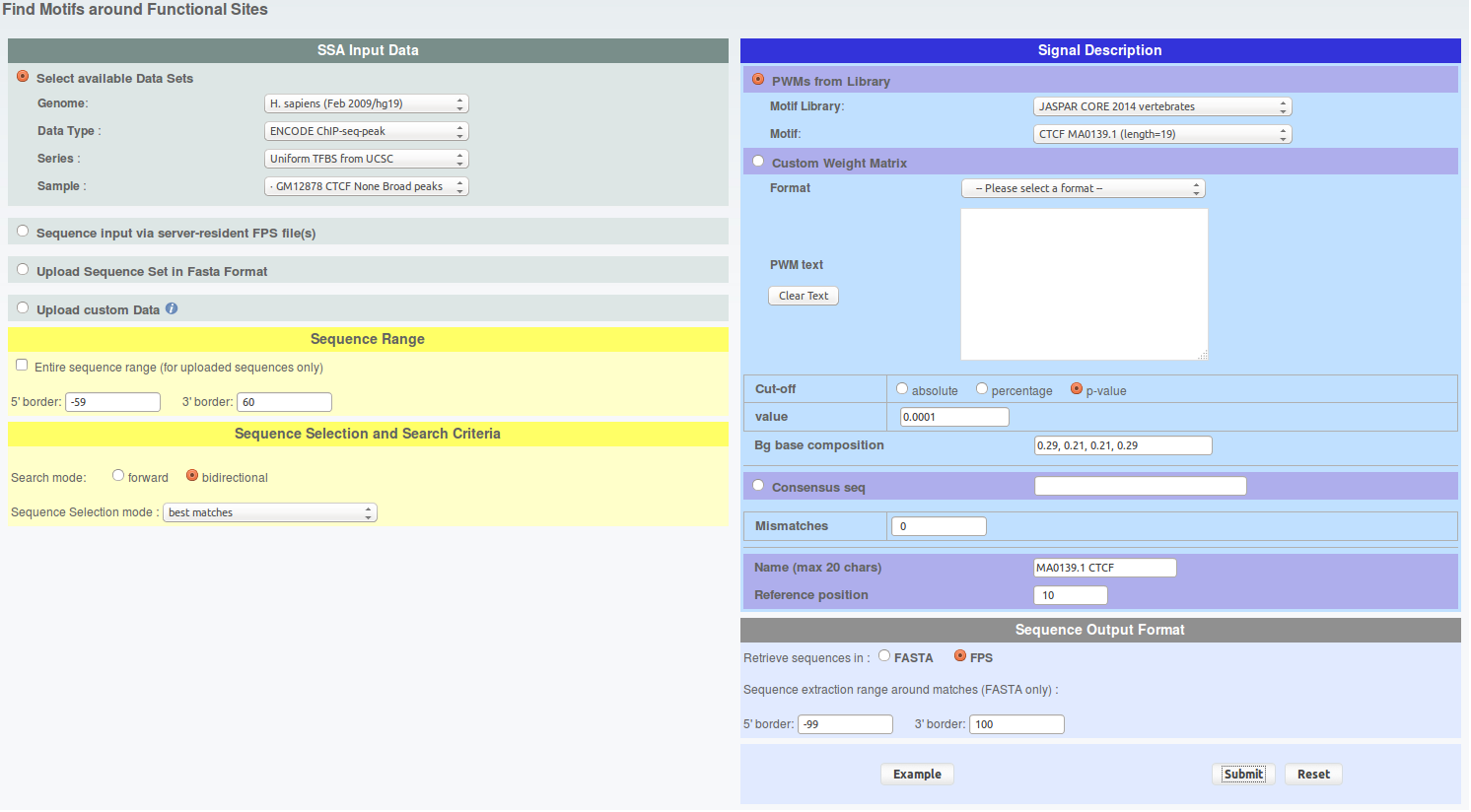
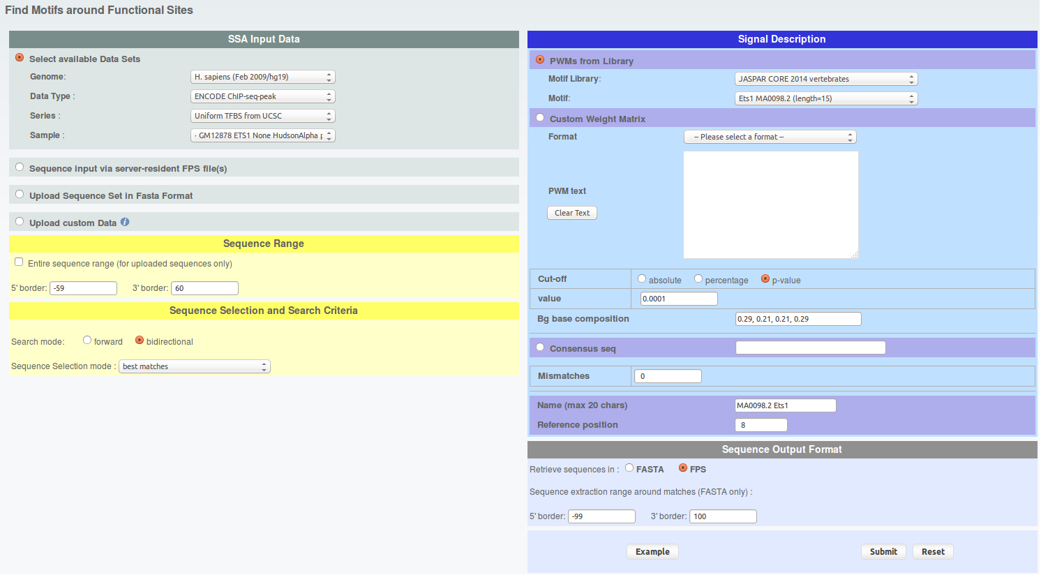
1. First, let's extract CTCF and ETS1 peaks which have CTCF and ETS1 binding motif nearby, respectively. To do this, go the FindM and fill the parameters as follows:

   click to show/hide FindM parameters.
   

   From the result page you will need to do two things. First save the results on your hard drive under sga format and name the files 'findm_CTCF.sga' and 'findm_ETS1.sga' (in case you can retrieve these files here : findm_CTCF.sga findm_ETS1.sga). Second, redirect the results toward ChIP-Extract by clicking on the corresponding button under 'Useful links for Downstream Analysis'.

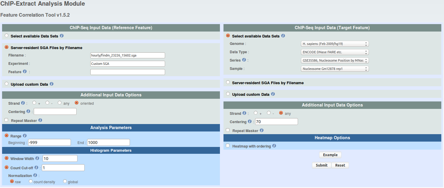
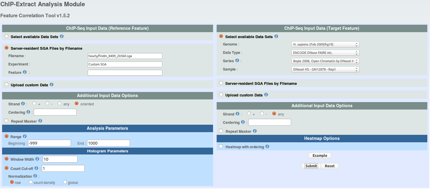
2. For each FindM result, run ChIP-extracts (4 runs total) as shown under and save ChIP-Extract results on your hard drive by naming your files 'chipextract_CTCF_MNase.mat','chipextract_CTCF_DNaseI.mat', 'chipextract_ETS1_MNase.mat', 'chipextract_ETS1_DNaseI.mat'.

   click to show/hide ChIP-Extract parameters.
   

3. Now open a R session in the folder where you have saved all the files and load the ChIP-Extract data.
   click to show/hide R code.

   
   # load needed functions
   source("em_api.R")
   
   # load data
   CTCF.MNase = as.matrix(read.table("chipextract_CTCF_MNase.mat"))
   CTCF.DNaseI = as.matrix(read.table("chipextract_CTCF_DNaseI.mat"))
   ETS1.MNase = as.matrix(read.table("chipextract_ETS1_MNase.mat"))
   ETS1.DNaseI = as.matrix(read.table("chipextract_ETS1_DNaseI.mat"))
   
   

4. To verify whether CTCF has nicely phased nucleosomes arrays on each sides of its binding sites, and that ETS1 does not, you can draw aggregation plots. An aggregation plot is the type of plot that ChIP-cor returns you. ChIP-Extract data can be used to draw exactly the same plots as you would have had with ChIP-Cor.
   click to show/hide R code.

   dist = seq(from=-990, to=990, by=10)
   xlab = "Dist to peak"
   ylab = "Norm. signal"
   
   # CTCF
   plot(dist, colSums(CTCF.MNase) / max(colSums(CTCF.MNase)), ylim=c(0,1), type='l', lwd=2, main="CTCF", xlab=xlab, ylab=ylab)
   lines(dist, colSums(CTCF.DNaseI) / max(colSums(CTCF.DNaseI)), ylim=c(0,1), lwd=2, lty=2)
   
   # ETS1
   plot(dist, colSums(ETS1.MNase) / max(colSums(ETS1.MNase)), ylim=c(0,1), type='l', lwd=2, main="ETS1", xlab=xlab, ylab=ylab)
   lines(dist, colSums(ETS1.DNaseI) / max(colSums(ETS1.DNaseI)), ylim=c(0,1), lwd=2, lty=2)
   
   # overlap
   plot(dist, colSums(CTCF.MNase) / max(colSums(CTCF.MNase)), ylim=c(0,1), type='l', lwd=2, main="CTCF", xlab=xlab, ylab=ylab)
   lines(dist, colSums(CTCF.DNaseI) / max(colSums(CTCF.DNaseI)), lwd=2, lty=2)
   lines(dist, colSums(ETS1.MNase) / max(colSums(ETS1.MNase)), lwd=2, lty=1, col='red')
   lines(dist, colSums(ETS1.DNaseI) / max(colSums(ETS1.DNaseI)), lwd=2, lty=2, col='red')
   legend("topright", legend=c("CTCF Mnase", "CTCF DNaseI", "ETS1 Mnase", "ETS1 DNaseI"), col=c("black", "black", "red", "red"), lwd=c(2,2,2,2), lty=c(1,2,1,2))
   
   xlab = ylab = NULL
   
   

   On the plots, a few things are visible. First, CTCF has a strong perdiodic MNase signal around its binding sites. This reflects the presence of well positioned nuclesomes (the peaks are ~140bp wide, a nucleosome core particule covers ~146bp). This is not the case for ETS1 albeit a weak periodic signal is visible. Second, in both cases, there is a clear drop of MNase signal at the binding site. This makes sense if we consider that a DNA binding factor needs the DNA to be accessible in order to bind it. Third, there is a DNaseI hypersensitivity at the level of CTCF and ETS1 binding sites. This reflects a more accessible chromatin structure at the level of the binding site and coroborate what is visible at the nucleosome level. If you look more carefully, you will see a decrease of DNaseI signal exactly on the binding site, which reflects the presence of the factor on the DNA (which impedes DNA accessibility and its digestion by DNaseI). This mark is called a footprint.

5. Now, let's run the EM partitioning to classify MNase signal and highlight whether different types of nucleosome organization are present in the data. We will allow the algorithm to shift and flip the data.
   Nucleosome signal is perdiodic by nature. Allowing the vectors to be phased by shifting them will increase the resolution of the signal. For instance, if the nucleosomes are not always organized the same around the binding site, this can create interference and mess up the nucleosome signal. Hopefully, this can be fixed by allowing shifting. Additionally, allowing algorithm to flip the vector might help resolving symetrical patterns which may originate from the overlap of two asymetrical anti-sense patterns.
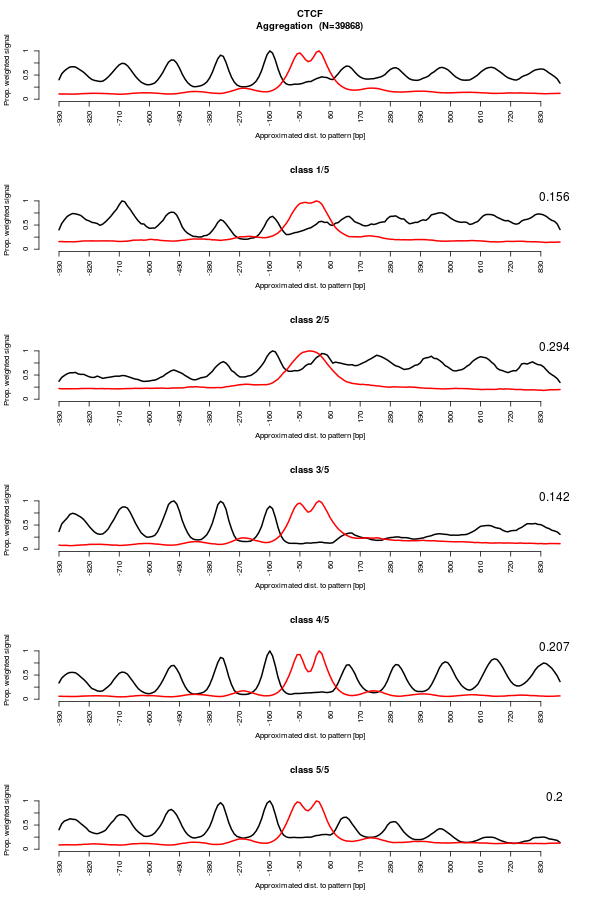
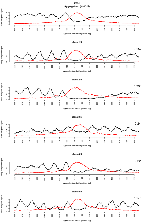
   click to show/hide R code.

   # All the functions are defined in em_api.R and are commented if needed
   
   # EM parameters
   n.class = 5
   n.iter = 5
   n.shift = 15
   seeding = "random"
   
   # plotting parameters
   lty = c(1,1)
   lwd = c(2,2)
   col = c("black", "red")
   
   # remove rows containing no MNase counts
   CTCF.filter = which(apply(CTCF.MNase, 1, sum) == 0)
   ETS1.filter = which(apply(ETS1.MNase, 1, sum) == 0)
   CTCF.MNase = CTCF.MNase[-CTCF.filter,]
   CTCF.DNaseI = CTCF.DNaseI[-CTCF.filter,]
   ETS1.MNase = ETS1.MNase[-ETS1.filter,]
   ETS1.DNaseI = ETS1.DNaseI[-ETS1.filter,]
   
   # em classification with flip and shift of MNase signal
   set.seed(1)
   CTCF.FLIP.SHIFT.prob = em.shape.shift.flip(CTCF.MNase, k=n.class, iter=n.iter, shift=n.shift, seeding=seeding)
   set.seed(1)
   ETS1.FLIP.SHIFT.prob = em.shape.shift.flip(ETS1.MNase, k=n.class, iter=n.iter, shift=n.shift, seeding=seeding)
   
   # plots the results, overlap DNaseI data (flipped and shifted accordingly to MNase)
   # two figures should appear in your working directory
   em.plot.class.profile(list(CTCF.MNase, CTCF.DNaseI), CTCF.FLIP.SHIFT.prob[[1]], "CTCF", sprintf("CTCF_%dclass_flip_%dshift_random.png", n.class, n.shift), n.iter, n.shift, flip=T, dist, lty, lwd, col)
   em.plot.class.profile(list(ETS1.MNase, ETS1.DNaseI), ETS1.FLIP.SHIFT.prob[[1]], "ETS1", sprintf("ETS1_%dclass_flip_%dshift_random.png", n.class, n.shift), n.iter, n.shift, flip=T, dist, lty, lwd, col)
   
   # dumps the probability arrays to hard drive, two rds files should appear in your working directory
   em.write.prob(CTCF.FLIP.SHIFT.prob[[1]], file=sprintf("CTCF_%dclass_flip_%dshift_random.rds", n.class, n.shift))
   em.write.prob(ETS1.FLIP.SHIFT.prob[[1]], file=sprintf("ETS1_%dclass_flip_%dshift_random.rds", n.class, n.shift))
   CTCF.FLIP.SHIFT.prob = ETS1.FLIP.SHIFT.prob = NULL
   
   

   click to show/hide the figures.

   The result figures shows a few interesting things.
   Regarding CTCF, a strong periodic MNase signal is still visible. Some classes are asymetric, suggesting that the CTCF sites may have an orientation. Moreover, the different classes show pretty different patterns, supporting different type of nucleosome organization around CTCF binding sites. Interestingly, the DNaseI footprint is still visible which indicates that the data were not shifted too much. This suggests that the nucleosomes are organized with respect to the binding sites (or a feature really close).
   Regarding ETS1, we now see nucleosomes clearly visible. However, in contrast to CTCF, DNaseI footprint dissapeared and the DNaseI hypersentitivty region is now wider. This reflects the fact that the MNase data vectors have been shifted. This means that the first nucleosome is not a constant distance from the binding site. This suggests that the nucleosomes are not organized with respect to the binding sites. Additionally, unlike what the aggregation plot was showing, the nucleosome organization around ETS1 binding sites is not anymore symetrical. For instance, class 1 and 3 have a nucleosome array on one side of the binding site only.

6. This algorithm performs a probabilistic (or soft) classification. This means that each binding site is assigned to all classes at the same time, with different probabilities. Nonetheless, it is still possible to extract all binding sites which have been assigned to a class, with a given minimal probability. Interestingly, it is also possible to update the original binding site position to take into account the shift and flip performed by the algorithm. In case, you can download the classification result file here : CTCF_5class_flip_15shift_random.rds ETS1_5class_flip_15shift_random.rds
   We know that ETS1 is a factor that mostly bind near TSS. Class 1 shows a profile which is compatible with this. The nucleosome array might reflect the nucleosomes downstream the TSS with the commonly described nucleosome depleted region near the TSS. Let's extract the binding sites which have been classified has belonging to class 1 with an overall probability of 0.9 or higher.
   click to show/hide R code.

   prob = 0.9
   class = 1
   bin.size = 10 # 10bp, value used in ChIP-Extract
   
   # reload probability array
   ETS1.FLIP.SHIFT.prob = em.read.prob("ETS1_5class_flip_15shift_random.rds")
   # load original ETS1 peak file
   ETS1.sga = read.table("findm_ETS1.sga", stringsAsFactors=F)
   
   # remove TFBS which were not containing MNase counts in the ChIP-Extract matrix, as above
   ETS1.sga = ETS1.sga[-ETS1.filter,]
   
   # extract TFBS coordinates and save them as SGA, this should make an sga file appear in your working directory
   em.extract.unoriented.sga.class.max(ETS1.sga, ETS1.FLIP.SHIFT.prob, sprintf("findm_ETS1_EM_class%d.sga", class), bin.size=bin.size, shift=n.shift, flip=T, class=class, threshold=prob)
   prob = class = bin.size = NULL
   ETS1.MNase = CTCF.MNase = ETS1.DNaseI = CTCF.DNaseI = NULL
   
   

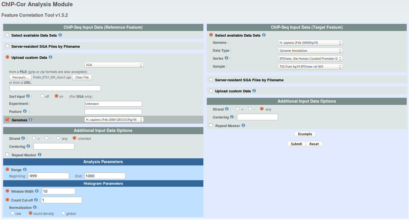
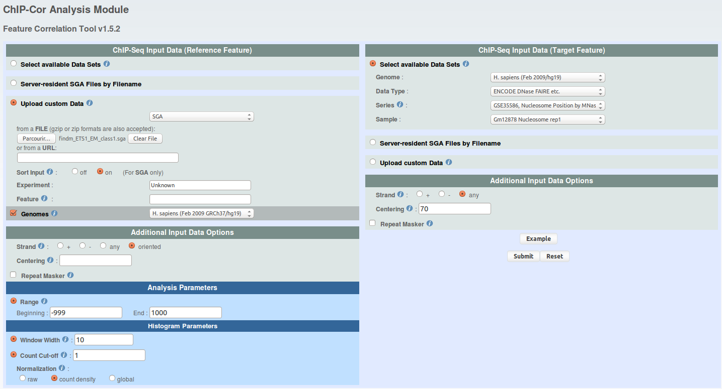
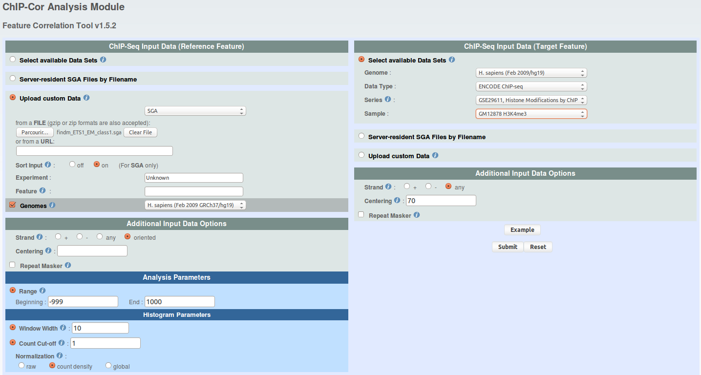
7. Now, go on ChIP-Cor, upload the coordinates extracted from class 1 and run ChIP-cor 3x as indicated under and save the results in the files named as follows : 'findm_ETS1_EM_class1_TSS.dat', 'findm_ETS1_EM_class1_MNase.dat', 'findm_ETS1_EM_class1_H3K4me3.dat'

   click to show/hide ChIP-Cor parameters.
   

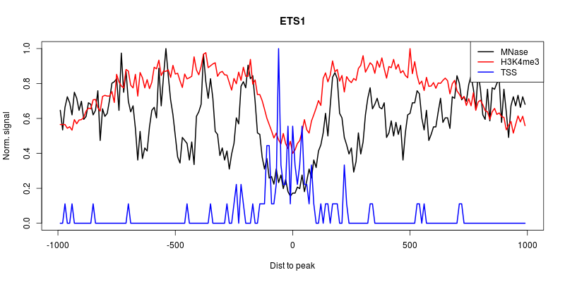
8. Go back to your R session and draw an aggregation plots with all the ChIP-Cor data.
   click to show/hide R code.

   # load ChIP-Cor data
   ETS1.TSS = read.table("findm_ETS1_EM_class1_TSS.dat")
   ETS1.MNase = read.table("findm_ETS1_EM_class1_MNase.dat")
   ETS1.H3K3me3 = read.table("findm_ETS1_EM_class1_H3K4me3.dat")
   
   # plot chipcor data
   xlab = "Dist to peak"
   ylab = "Norm. signal"
   plot(ETS1.MNase[,1], ETS1.MNase[,2] / max(ETS1.MNase[,2]), ylim=c(0,1), type='l', lwd=2, main="ETS1 class 1", xlab=xlab, ylab=ylab)
   lines(ETS1.H3K3me3[,1], ETS1.H3K3me3[,2] / max(ETS1.H3K3me3[,2]), ylim=c(0,1), lwd=2, lty=1, col="red")
   lines(ETS1.TSS[,1], ETS1.TSS[,2] / max(ETS1.TSS[,2]), ylim=c(0,1), lwd=2, lty=1, col="blue")
   legend("topright", legend=c("MNase", "H3K4me3", "TSS"), lwd=c(2,2,2), lty=c(1,1,1), col=c("black", "red", "blue"))
   
   

   click to show/hide the figure.

   
   The peak of TSS density in the nucleosome depleted region together with the H3K4me3 labelling suggest that the binding sites which have been assigned to this class are indeed in promoters regions. However, the exact orientation of these promoters is hard to estimate since H3K4me3 labelling is pretty symetrical and that we can see nucleosomes on both sides of the TSS density peak.
   Now, you might want to pursue this analysis by extracting other classes coordinates or to rerun an entire analysis on other type of data such as histone marks.
   

Part IV: H3K4me3 around human promoters. Dataset in this example is from GEO series GSE29611 and EPD.

We will use ChIP-Extract Analysis Module to generate a tag count matrix in defined bins around promoters. Select appropriate target feature and then click submit.

• Reference feature: hg19; Genome Annotation; EPDNew; rel 003
• Target feature: hg19; ENCODE ChIP-seq; GSE29611; GM12878 H3K4me3
• Analysis parameters: -1000 to 1000; Window width:10; Count cut-off:10

Download the Ref SGA File and Table (TEXT) and save as promoters.sga and h3k4me3_promoters.txt respectively.

Perform iterative shape based partitioning with shifting and write class output as sga files. R script Hide script

Read data:

data = as.matrix(read.table("h3k4me3_promoters.txt"))

Define classes and shifts:

K=4; S=3; N=dim(data)[1]; L=dim(data)[2]-S+1; ITER=5 

Iterative shape based partitioning with shifting

mean_shift=floor(S/2)+1
  c    = colMeans(data[,mean_shift:(mean_shift+L-1)])
  flat = matrix(data=mean(data), nrow=1, ncol=L)
  q=q0 = dnorm(1:S,mean_shift,1)/sum(dnorm(1:S,mean_shift,1))

  for (m in 1:(K-1)) {
     c = rbind(flat,c)
     q = rbind(q0/m,q); q/sum(q)

     for(i in 1:ITER) {
        reg_shift(q); em_shape_shift(c,q,data); plot_classes(c); print(q)}
     }

Extract class labels

class=apply(apply(p,c(1,2),sum),1,order)[4,]

Write output sga files for different classes

peak <- read.table("promoters.sga", header=F, sep="\t")
write.table(peak[which(class==1),], "h3k4me3_class1.sga", sep="\t", quote=F, row.names=F, col.names=F)
write.table(peak[which(class==2),], "h3k4me3_class2.sga", sep="\t", quote=F, row.names=F, col.names=F)
write.table(peak[which(class==3),], "h3k4me3_class3.sga", sep="\t", quote=F, row.names=F, col.names=F)
write.table(peak[which(class==4),], "h3k4me3_class4.sga", sep="\t", quote=F, row.names=F, col.names=F)

Now you may want to explore these four classes in-terms of associated features, such as PolII, conservation, or check the enrichment for various core promoter motifs (TATA, CCAAT-box, etc).